tigue.com

Whiteboarder: A Two Bit Image Processor

May 26, 2020
header  

Whiteboarder is a two bit image processor, tuned for whiteboard captures. The four most common dry erase marker colors are recognized: black, red, green, and blue. Four colors, ergo two bit color images.

brightfield cuboid packager  

I have long wanted a tool dedicated to cleaning up whiteboard capture images. There are commercial tools but nothing made me happy. Of late I’ve been coding a lot of image processing in a machine learning context. So, Whiteboarder just kinda happened over this last month by hacking on a Jupyter notebook to see what could be cooked up with the tools I was already using for a different purpose.

red kneecap  

Note: this is very much not an end-user tool. The tech is simply not mature enough for full auto-pilot. But the results can be impressive with a touch of human intelligence in the mix. So, Whiteboarder is for folks who are comfortable seeing what is going on under the hood. There will be code.

git and jupyter book  

Additionally, the project is an experiment with Jupyter as a development platform. The question is: just how far can a Jupyter notebook’s UI be morphed into an end-user-ish utility tool? The code is available on GitHub.

Whiteboard can read your own images: specify an URL, upload a file, or take a picture in-browser. To take Whiteboarder for a test drive on Colab click below:

Eight Bit Gauges in Jupyter

April 27, 2020

Over the last few weeks I have written so many variants on “eight bit gauges” in Jupyter that I thought I might as well corral them all together in a menagerie. By eight big gauges I mean histograms with 256 bins.

For example, the above image is for grayscale images as implied by the gray gradient on the face of the histogram. The red line is the same data but as a cumulative distribution, starting at zero and marching monotonically to 100% total luminance.

range selector The code is all Python using common plotting libraries (Bokeh, Plotly, Matplotlib, etc.). In particular, the code has been well tested on Colab, including working out full-screenable versions which perform well as “slides.” I’ve licensed the code under the Apache 2 license. So, peruse the menagerie and maybe take one home.

simple wide

There is a pre-run and runnable copy on Colab, eight_bit_gauges.ipynb, which can also be found on GitHub in the shell repo. To load it from from GitHub and run your own copy:

Jupyter Books' Many Manifestations of a Notebook

March 03, 2020

four reps of ipynb

This is an addendum to my 2020-01 post entitled, Jupyter Book to Colab.

Jupyter Book is a tool which generates static HTML renderings of Jupyter .ipynb files. It can optionally generate links to live Python kernels which can run the code in the original .ipynb files. This is called the “interact” button.

In my earlier post I described how I extended the interact button to work with Colab rather than one of Jupyter Books’ already built-out interacts to Jupyer services (e.g. Binder).

While discussing this little hack, I have found this whiteboard sketch helps explain what is going on under the hood. In the context of Jupyter-Book-interact-Colab deploy, any given Jupyter notebook .ipynb file can have four manifestions.

Let’s walk through the five steps.

1. The source notebook at home

A git repository is archived somewhere, say, Microsoft GitHub (but it could be any git repo). In the context of this post the repo is one built out to work with Jupyter Book, which means is it essentially just a collection of Jupyter notebooks and markdown files.

2. Pre-run notebook as HTML

For step 2, the repo has been fetched from GitHub and run through Jupyter Book with the output being a bunch of static web content (HTML, JavaScript, CSS, and images).

Static web sites are the simplest kind of web site: they are simply file servers talking HTTP. In this diagram the example static site is http://static-bar.com.

3. Hand off to Colab

This is what in Jupyter Book is referred to as interacting, moving from a static web page rendering of an (optionally pre-run) notebook to something backed by a live Jupyter kernel. Normally, Jupyter Book will hand off to Binder for provisioning Jupyter kernels. In my hack, open source Binder is replaced with commercial Google Colab.

The hand off is simply an http:// URL to Colab, which includes/ends-with a map to the .ipynb file that Colab should load from GitHub. That mapping will result in an URL of the form:

https://colab.research.google.com/github/my_org/my_repo/blob/my_branch/my_file.ipynb

4. Colab kernel spin-up

Next, the web browser follows the http://colab.research.google.com URL, loading a new web page. At Colab, an HTTP GET arrives and the URL is parsed. When colab sees the /github/ part, it knows that the user is requesting that an .ipynb file be fetched from GitHub. The tail of the URL provides the organization, repo name, and relative file path. Colab then fetches the specified file from github.com.

Behind the scene Colab spins up a new virtual machine to provide a Jupyter kernel for the request. (Anyone with a gMail email address can have up to two VMs running simultaneously.)

Eventually (quickly) the HTTP response goes down to the browser where the user sees the notebook and can run the code.

5. Persisting a modified version

“Playground mode” is the Colab term for a transient, unpersisted version of a notebook running in a Colab VM. If a reader wants to play with and run the code (read: modify the input notebook) and keep a copy, exiting playground mode will save a copy of the modified .ipynb in the users Google Drive.

The take away is that open source tools make it possible to have a static web site showing HTML rendering of .ipynb files. Those static HTML files can then link to Colab (or Binder) to on-demand hook the notebook up to a new VM. A static web site linking to free compute.

Traing Data for Neuron Reconstructors

January 27, 2020

651806289 MinIP

The Cell Types Database is one of the major data products of The Allen Institute for Brain Science. In the Cell Types project, the Allen is constructing an altas of all type of cells found in brains of mice and humans.

There are multiple ways different cells are represented in the Database: electrophysiology spike train recordings, simulation models (GLIF or perisomatic), etc. Of particular interest for the Reconstrue project is the morphology data – the skeletons in the *.swc files.

The Allen has created about 500 SWC files for mouse neurons. In the following Venn diagram of all The Allen’s mouse cells, those ~500 SWC files are grouped inside the red circle.

The main problem from The Allen’s perspective is that they would like to have the red circle be as big as the main outer circle. Each SWC files represents many hours of manual labor by trained specialists reviewing and editing the SWC file. The Allen processes hundreds of such cells a year. Creating skeleton reconstructions is currently a serious manual labor bottleneck.

The header image of this post is an example brightfield imaged neuron from The Cell Types Database. This would seem like the sort of object recognition that CNNs and friends (RNNs, FFNs, U-Net, etc.) could automate. This is proving to be nontrivial.

Model training data

The image stack is the input to the machine to be built, and the SWC file is the output.

From a model training perspective, the skeleton in an SWC file can be seen as the “labels” (labeling each voxel in a volume as either inside or outside the cell) for “the training data” (read: the brightfield image stacks). As such, for the purpose of training reconstruction models, we’re only interested in the subset of cells in the atlas Cell Types Database that have skeletons and a microscopy image stack.

!pip install --quiet allensdk
# Query the Cell Types DB for files with skeletons a.k.a. reconstructions

# via https://allensdk.readthedocs.io/en/latest/cell_types.html#cell-types-cache
from allensdk.core.cell_types_cache import CellTypesCache

ctc = CellTypesCache(manifest_file='cell_types/manifest.json')

# a list of cell metadata for cells with reconstructions, download if necessary
cells = ctc.get_cells(require_reconstruction=True)
print('Number of cells with SWC files: %i' % len(cells))
Number of cells with SWC files: 637

Some of those are human cells, atop the roughly 500 mouse cells. Humans brains are much bigger than mouse brains. Training should focus on one species. The Allen has many more mouse neurons than human neurons. So, train on mouse neurons only.

from allensdk.api.queries.cell_types_api import CellTypesApi

# We want mouse cells that have images and skeletons, both.
# Former is data; latter is training labels a.k.a. gold standards.
cells = ctc.get_cells(require_reconstruction=True, require_morphology=True, species=[CellTypesApi.MOUSE])
print('Number of mouse cells with images and SWC files: %i' % len(cells))
Number of mouse cells with images and SWC files: 485

So, for brightfield reconstructor training, The Allen’s Cell Types Database can be used as a labeled training dataset consisting of about 500 samples. That’s somewhere on the order of ten petabytes of training data.

References

Cell Types DB Physiology and Morphology whitepaper

cell types cache docs.

Brightfield colormapping

January 20, 2020

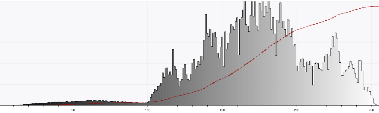
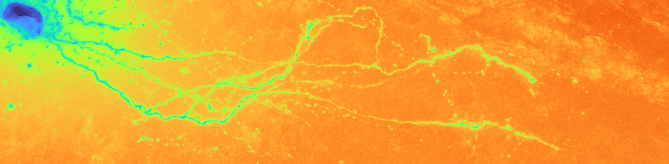
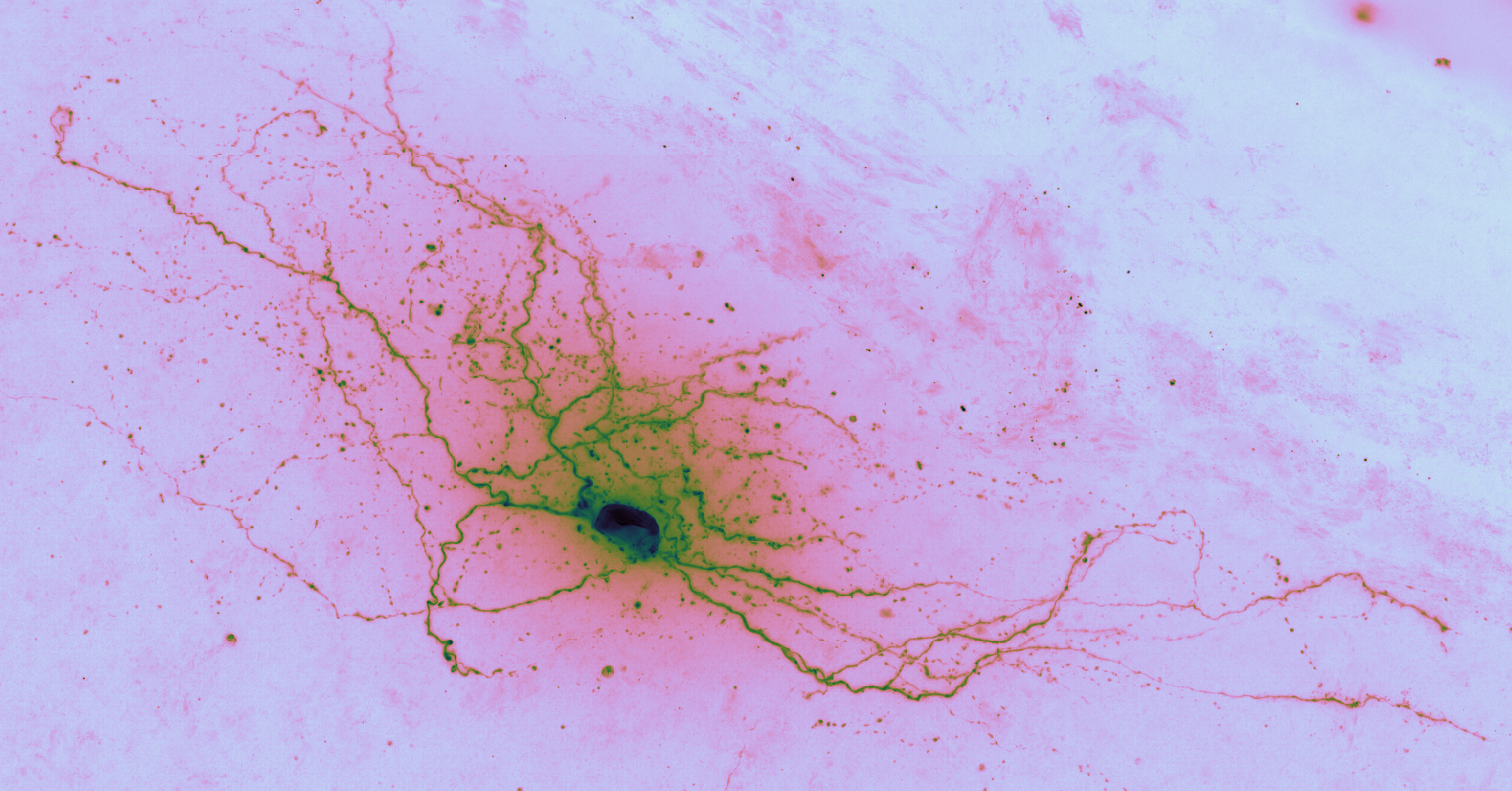
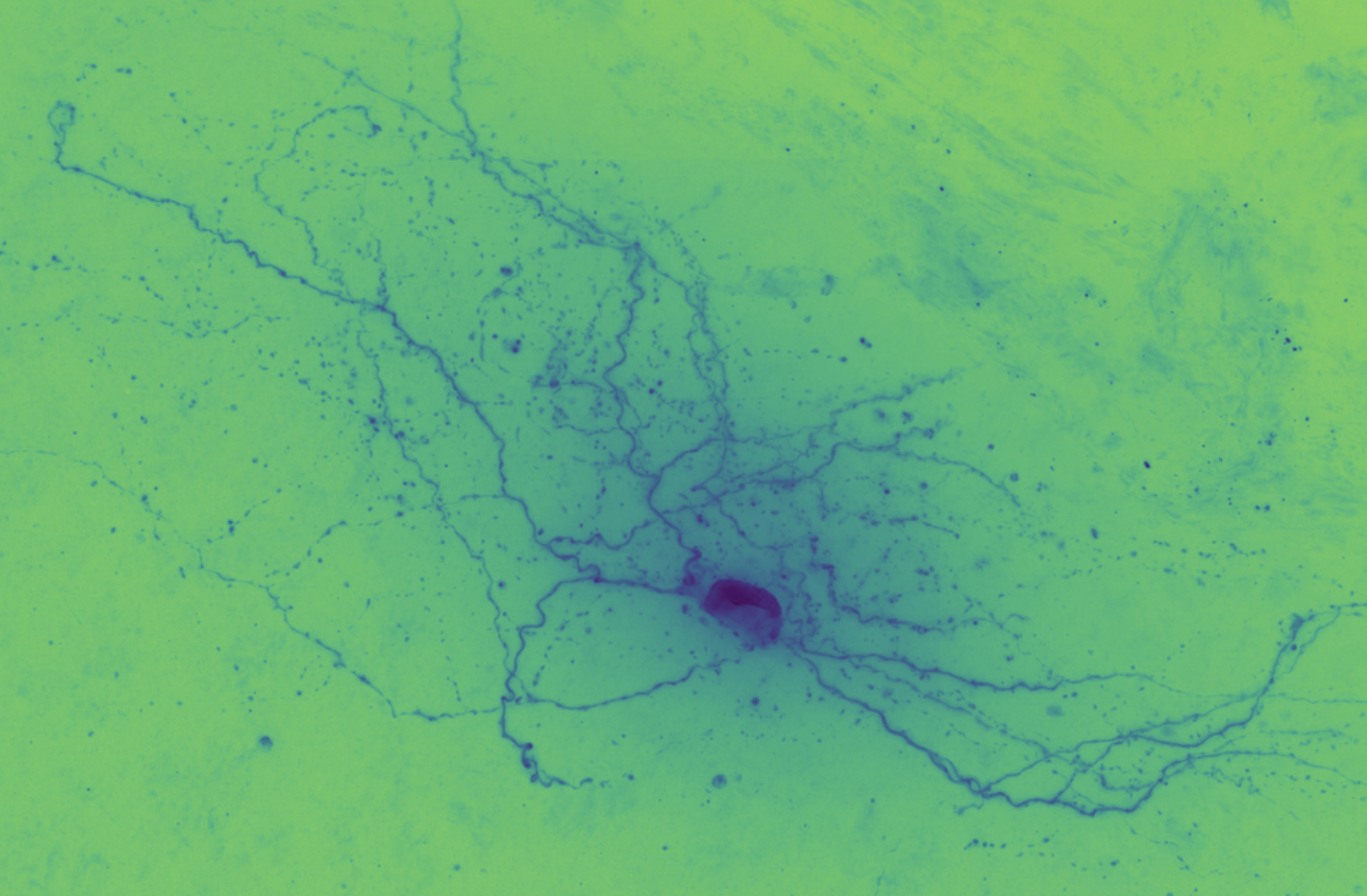
Brightfield data is single channel. It is not color data, which is triple band data (Red, Green, Blue or such). Therefore there is the opportunity to colorize the images according to some map. Pseudocoloring can be seen as some of the simpliest form of image processing for brightfield microscopy. As can be seen in this page’s header imageset, different colormaps bring out different features of an image.

The whole goal of this project is to make tools which make it easier to gain insights from the raw images off the microscope. Colormapping is about as basic as it gets but it should be addressed in the current Jupyter-based context of Python on the server and JavaScript on the client.

Colormaps

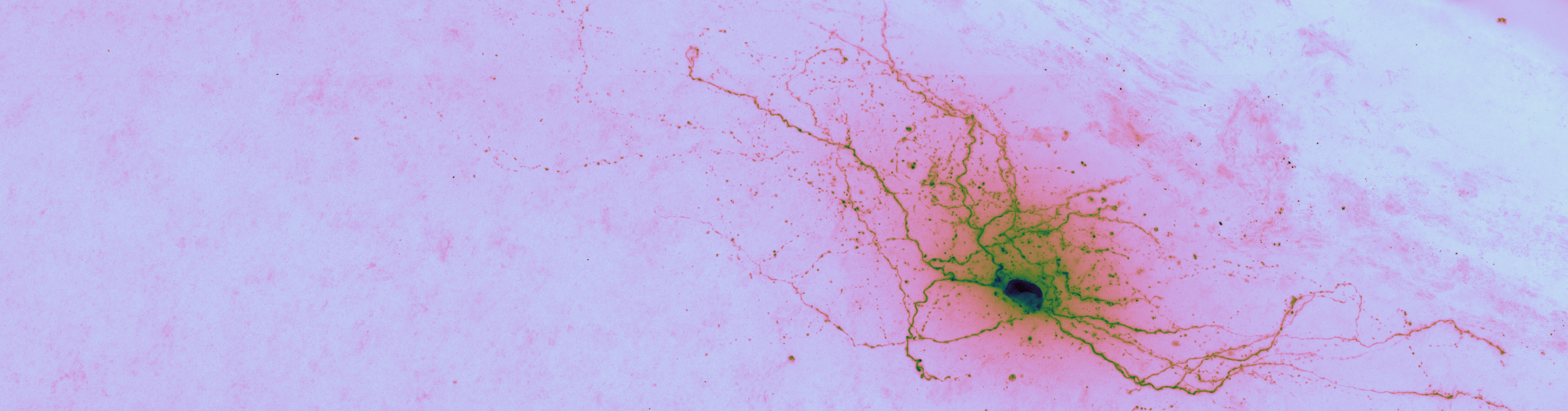
This code is being written in 2020 so let’s color these micrographs like it’s 2020, with decent color maps that work well with brihtfield images. In particular 2019 saw the publication of the Turbo colormap by Google AI which looks good – loud but effective at separating the foreground from backfield (e.g., it’s the reddish image at the top of this page).

Further, this codebase is Jupyter-based. As used in this project, that means Python on the Jupyter server and JavaScript in the browser. It would be nice to use the same colormaps in images produced by both Python and JavaScript. As such, this project has been built out using a few colormaps that seem to work well.

Jet => Turbo

Jet is the default “rainbow” colormap in Python-land. Jet is a lame implementation. There are other rainbow colormaps, say, Turbo.

Some folks really don’t like Jet. For example, How Bad Is Your Colormap? Or, Why People Hate Jet – and You Should Too:

The above article also has a useful snippet of code to test a colormap:

def grayify_cmap(cmap):
    """Return a grayscale version of the colormap"""
    cmap = plt.cm.get_cmap(cmap)
    colors = cmap(np.arange(cmap.N))
    
    # convert RGBA to perceived greyscale luminance
    # cf. http://alienryderflex.com/hsp.html
    RGB_weight = [0.299, 0.587, 0.114]
    luminance = np.sqrt(np.dot(colors[:, :3] ** 2, RGB_weight))
    colors[:, :3] = luminance[:, np.newaxis]
    
    return cmap.from_list(cmap.name + "_grayscale", colors, cmap.N)

Turbo

The Turbo colormap is a new and improved Jet, introduced in a mid-2019 Google AI blog post, Turbo, An Improved Rainbow Colormap for Visualization:

Turbo, a new colormap that has the desirable properties of Jet while also addressing some of its shortcomings, such as false detail, banding and color blindness ambiguity.

Turbo is a slot-in replacement for Jet, and is intended for day-to-day tasks where perceptual uniformity is not critical, but one still wants a high contrast, smooth visualization of the underlying data.

The following juxtaposition illustrates Jet’s flaws (images are from Google’s post).

Turbo:

Jet:

In a simulated 3D environment (Turbo on the left, Jet on the right):

In an actually brightfield MinIP (Turbo on the left, Jet on the right):

So, it’s not a complete win but Turbo is easier to look at than Jet and brings out more features that Jet.

Turbo is not yet distributed with Python’s Matplotlib. But adding a new colormap for use by Matplotlib is only a handful of lines of code. At its core a Matplotlib colormap is just an array of 256 values, each a color (a RGB triplet) which Matplotlib wants normalized into a float between 0 and 1, rather than an 8-bit 0 to 255 range which is what HTML expects.

turbo_colormap_data = [[0.18995,0.07176,0.23217],[0.19483,0.08339,0.26149],[0.19956,0.09498,0.29024],[0.20415,0.10652,0.31844],[0.20860,0.11802,0.34607],[0.21291,0.12947,0.37314],[0.21708,0.14087,0.39964],[0.22111,0.15223,0.42558],[0.22500,0.16354,0.45096],[0.22875,0.17481,0.47578],[0.23236,0.18603,0.50004],[0.23582,0.19720,0.52373],[0.23915,0.20833,0.54686],[0.24234,0.21941,0.56942],[0.24539,0.23044,0.59142],[0.24830,0.24143,0.61286],[0.25107,0.25237,0.63374],[0.25369,0.26327,0.65406],[0.25618,0.27412,0.67381],[0.25853,0.28492,0.69300],[0.26074,0.29568,0.71162],[0.26280,0.30639,0.72968],[0.26473,0.31706,0.74718],[0.26652,0.32768,0.76412],[0.26816,0.33825,0.78050],[0.26967,0.34878,0.79631],[0.27103,0.35926,0.81156],[0.27226,0.36970,0.82624],[0.27334,0.38008,0.84037],[0.27429,0.39043,0.85393],[0.27509,0.40072,0.86692],[0.27576,0.41097,0.87936],[0.27628,0.42118,0.89123],[0.27667,0.43134,0.90254],[0.27691,0.44145,0.91328],[0.27701,0.45152,0.92347],[0.27698,0.46153,0.93309],[0.27680,0.47151,0.94214],[0.27648,0.48144,0.95064],[0.27603,0.49132,0.95857],[0.27543,0.50115,0.96594],[0.27469,0.51094,0.97275],[0.27381,0.52069,0.97899],[0.27273,0.53040,0.98461],[0.27106,0.54015,0.98930],[0.26878,0.54995,0.99303],[0.26592,0.55979,0.99583],[0.26252,0.56967,0.99773],[0.25862,0.57958,0.99876],[0.25425,0.58950,0.99896],[0.24946,0.59943,0.99835],[0.24427,0.60937,0.99697],[0.23874,0.61931,0.99485],[0.23288,0.62923,0.99202],[0.22676,0.63913,0.98851],[0.22039,0.64901,0.98436],[0.21382,0.65886,0.97959],[0.20708,0.66866,0.97423],[0.20021,0.67842,0.96833],[0.19326,0.68812,0.96190],[0.18625,0.69775,0.95498],[0.17923,0.70732,0.94761],[0.17223,0.71680,0.93981],[0.16529,0.72620,0.93161],[0.15844,0.73551,0.92305],[0.15173,0.74472,0.91416],[0.14519,0.75381,0.90496],[0.13886,0.76279,0.89550],[0.13278,0.77165,0.88580],[0.12698,0.78037,0.87590],[0.12151,0.78896,0.86581],[0.11639,0.79740,0.85559],[0.11167,0.80569,0.84525],[0.10738,0.81381,0.83484],[0.10357,0.82177,0.82437],[0.10026,0.82955,0.81389],[0.09750,0.83714,0.80342],[0.09532,0.84455,0.79299],[0.09377,0.85175,0.78264],[0.09287,0.85875,0.77240],[0.09267,0.86554,0.76230],[0.09320,0.87211,0.75237],[0.09451,0.87844,0.74265],[0.09662,0.88454,0.73316],[0.09958,0.89040,0.72393],[0.10342,0.89600,0.71500],[0.10815,0.90142,0.70599],[0.11374,0.90673,0.69651],[0.12014,0.91193,0.68660],[0.12733,0.91701,0.67627],[0.13526,0.92197,0.66556],[0.14391,0.92680,0.65448],[0.15323,0.93151,0.64308],[0.16319,0.93609,0.63137],[0.17377,0.94053,0.61938],[0.18491,0.94484,0.60713],[0.19659,0.94901,0.59466],[0.20877,0.95304,0.58199],[0.22142,0.95692,0.56914],[0.23449,0.96065,0.55614],[0.24797,0.96423,0.54303],[0.26180,0.96765,0.52981],[0.27597,0.97092,0.51653],[0.29042,0.97403,0.50321],[0.30513,0.97697,0.48987],[0.32006,0.97974,0.47654],[0.33517,0.98234,0.46325],[0.35043,0.98477,0.45002],[0.36581,0.98702,0.43688],[0.38127,0.98909,0.42386],[0.39678,0.99098,0.41098],[0.41229,0.99268,0.39826],[0.42778,0.99419,0.38575],[0.44321,0.99551,0.37345],[0.45854,0.99663,0.36140],[0.47375,0.99755,0.34963],[0.48879,0.99828,0.33816],[0.50362,0.99879,0.32701],[0.51822,0.99910,0.31622],[0.53255,0.99919,0.30581],[0.54658,0.99907,0.29581],[0.56026,0.99873,0.28623],[0.57357,0.99817,0.27712],[0.58646,0.99739,0.26849],[0.59891,0.99638,0.26038],[0.61088,0.99514,0.25280],[0.62233,0.99366,0.24579],[0.63323,0.99195,0.23937],[0.64362,0.98999,0.23356],[0.65394,0.98775,0.22835],[0.66428,0.98524,0.22370],[0.67462,0.98246,0.21960],[0.68494,0.97941,0.21602],[0.69525,0.97610,0.21294],[0.70553,0.97255,0.21032],[0.71577,0.96875,0.20815],[0.72596,0.96470,0.20640],[0.73610,0.96043,0.20504],[0.74617,0.95593,0.20406],[0.75617,0.95121,0.20343],[0.76608,0.94627,0.20311],[0.77591,0.94113,0.20310],[0.78563,0.93579,0.20336],[0.79524,0.93025,0.20386],[0.80473,0.92452,0.20459],[0.81410,0.91861,0.20552],[0.82333,0.91253,0.20663],[0.83241,0.90627,0.20788],[0.84133,0.89986,0.20926],[0.85010,0.89328,0.21074],[0.85868,0.88655,0.21230],[0.86709,0.87968,0.21391],[0.87530,0.87267,0.21555],[0.88331,0.86553,0.21719],[0.89112,0.85826,0.21880],[0.89870,0.85087,0.22038],[0.90605,0.84337,0.22188],[0.91317,0.83576,0.22328],[0.92004,0.82806,0.22456],[0.92666,0.82025,0.22570],[0.93301,0.81236,0.22667],[0.93909,0.80439,0.22744],[0.94489,0.79634,0.22800],[0.95039,0.78823,0.22831],[0.95560,0.78005,0.22836],[0.96049,0.77181,0.22811],[0.96507,0.76352,0.22754],[0.96931,0.75519,0.22663],[0.97323,0.74682,0.22536],[0.97679,0.73842,0.22369],[0.98000,0.73000,0.22161],[0.98289,0.72140,0.21918],[0.98549,0.71250,0.21650],[0.98781,0.70330,0.21358],[0.98986,0.69382,0.21043],[0.99163,0.68408,0.20706],[0.99314,0.67408,0.20348],[0.99438,0.66386,0.19971],[0.99535,0.65341,0.19577],[0.99607,0.64277,0.19165],[0.99654,0.63193,0.18738],[0.99675,0.62093,0.18297],[0.99672,0.60977,0.17842],[0.99644,0.59846,0.17376],[0.99593,0.58703,0.16899],[0.99517,0.57549,0.16412],[0.99419,0.56386,0.15918],[0.99297,0.55214,0.15417],[0.99153,0.54036,0.14910],[0.98987,0.52854,0.14398],[0.98799,0.51667,0.13883],[0.98590,0.50479,0.13367],[0.98360,0.49291,0.12849],[0.98108,0.48104,0.12332],[0.97837,0.46920,0.11817],[0.97545,0.45740,0.11305],[0.97234,0.44565,0.10797],[0.96904,0.43399,0.10294],[0.96555,0.42241,0.09798],[0.96187,0.41093,0.09310],[0.95801,0.39958,0.08831],[0.95398,0.38836,0.08362],[0.94977,0.37729,0.07905],[0.94538,0.36638,0.07461],[0.94084,0.35566,0.07031],[0.93612,0.34513,0.06616],[0.93125,0.33482,0.06218],[0.92623,0.32473,0.05837],[0.92105,0.31489,0.05475],[0.91572,0.30530,0.05134],[0.91024,0.29599,0.04814],[0.90463,0.28696,0.04516],[0.89888,0.27824,0.04243],[0.89298,0.26981,0.03993],[0.88691,0.26152,0.03753],[0.88066,0.25334,0.03521],[0.87422,0.24526,0.03297],[0.86760,0.23730,0.03082],[0.86079,0.22945,0.02875],[0.85380,0.22170,0.02677],[0.84662,0.21407,0.02487],[0.83926,0.20654,0.02305],[0.83172,0.19912,0.02131],[0.82399,0.19182,0.01966],[0.81608,0.18462,0.01809],[0.80799,0.17753,0.01660],[0.79971,0.17055,0.01520],[0.79125,0.16368,0.01387],[0.78260,0.15693,0.01264],[0.77377,0.15028,0.01148],[0.76476,0.14374,0.01041],[0.75556,0.13731,0.00942],[0.74617,0.13098,0.00851],[0.73661,0.12477,0.00769],[0.72686,0.11867,0.00695],[0.71692,0.11268,0.00629],[0.70680,0.10680,0.00571],[0.69650,0.10102,0.00522],[0.68602,0.09536,0.00481],[0.67535,0.08980,0.00449],[0.66449,0.08436,0.00424],[0.65345,0.07902,0.00408],[0.64223,0.07380,0.00401],[0.63082,0.06868,0.00401],[0.61923,0.06367,0.00410],[0.60746,0.05878,0.00427],[0.59550,0.05399,0.00453],[0.58336,0.04931,0.00486],[0.57103,0.04474,0.00529],[0.55852,0.04028,0.00579],[0.54583,0.03593,0.00638],[0.53295,0.03169,0.00705],[0.51989,0.02756,0.00780],[0.50664,0.02354,0.00863],[0.49321,0.01963,0.00955],[0.47960,0.01583,0.01055]]
turbo_cmap=ListedColormap(turbo_colormap_data) #ListedColormap is a Matplotlib thing

Viridis

Viridis is the default colormap for Matplotlib. It doesn’t suck.

Cubehelix

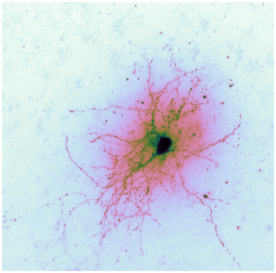
Cubehelix is a modern colormap that works well with brightfield because the top end of the colormap fades out to white, much like the bright field in brightfield.

“Cubehelix was created to vary smoothly in both lightness and hue, but appears to have a small hump in the green hue area.” Seems to be a 2011 thing out of the astronomy world.

In the end, Turbo seems like a good default.

Jupyter Book to Colab

January 07, 2020

jupyter book to colab

Like any developer with a blog, I occasionally talk about blog tooling. Sorry. I just went through ye olde blog overhaul for the first time in years, so the sensitive should stop reading now and the rest of you have been warned. Stick around for a short story about a small “good” hack for blogging about Jupyter notebooks.

Introduction

Static Site Generators (SSGs) have been around for a while and are the bee’s knees. But now they are becoming the next generation markdown files – the front end explorable explanations to repos, which can optionally be wired up to kernel VMs for execution by the more curious reader.

For this rebuild, I used two SSGs: Gatsby and Jupyter Book. The Gatsby part is just another story of a classic Jekyll to Gatsby migration so let’s not talk about it.

The other part of the SSG story is about Jupyter Book, which is used in the rebuild to SSG git repos that are full of Jupyter notebook *.ipynb files. This is the part of the story that is interesting because it is about emerging tech, to be described herein.

The novelty

I’m only going to go over the truly novel bit, which as the title implies is the integration of Jupyter Book and Google’s Colab, their free Jupyter hosting service. That is, Jupyter Book renders Jupyter notebook files (*.ipynb) for static hosting on tigue.com. Additionally, links into Colab are made available to spin up a kernel VM for any reader wishing to execute a notebook they read on tigue.com.

The contextual goal is a static site for a software developer. The site’s front consists of a blog and set of projects. The latter involves a lot of Jupyter notebooks, which are static hostly on the static site as HTML snapshots of pre-run notebooks. Additionally, reader can easily execute the notebooks, without any admin hassles nor costs for me, by clicking through to Google Colab.

The “clicking through to Google Colab” hack is the novel bit. Jupyter Book usually clicks through to JupyterHub or Binder via the Interact buttons on the top of the page, not to Colab.

(Of course, if executing on Colab, it would be really helpful and more interesting if those notebooks being clicked through to had been previously tested to run on Colab; but that topic is out of the scope of this post.)

Context

I’ve been a long time believer in static site generators (SSGs). For this blog rebuild, I’m using two SSG tools: Gatsby and Jupyter Book. I use Gastby to SSG the blog, and I use Jupyter Book to SSG repos of notebook which act as the demo/web presence for the code projects. The SSG notebooks have links into Google Colab if folks want to actually run a given notebook on a VM, rather than just read a static notebook rendering.

Gatsby was the obvious choice since I’ve been using React and GraphQL for a while now. And Jupyter Book is simply the best in class for its task (notebook SSGing). I can report that SSG tooling has come along nicely over the last few years.

Jupyter Book generates the “static site” for a given git repo full of notebooks (*.ipynb files). The static site will have pre-run notebook web pages i.e. cell outputs will be included to demonstrate what the software can do.

Additionally if the reader wishes they can interact with the notebook: a link in the Jupyter Book generated notebook pages will have a link to Colab which will grab the notebook clean from GitHub and provision a virtual machine within which to run and interact with the notebook.

Combined these two SSG tools enable a projects-and-blog web presence for a developer to be run completely staticly, without involving say Medium for blog hosting and MSFT GitHub for notebook rendering, yet code can also be run “dynamically” on Colab. It makes for a low hassle yet high functionality coder’s blog.

Interactivity for Jupyter Book

I want readers to be able to expeditiously run and interact with the code in said notebooks statically hosted on tigue.com. And I don’t want to manage that nor pay for the provioning of VMs, thank you very much. Google Colab fits the bill perfectly.

Jupyter Book has a lot of nice functionality already. I don’t know of a better equivalent. Nonetheless, for my React-based blog there is functionality overlap between Gatsby and Jupyter Book. E.g., the latter uses Jekyll for static page generation, which the former is also doing.

Conceivably, much of Jupyter Book could be reproduced by Gatsby. But Gatsby is JavaScript; that’s getting away from the Python world so it’s unlikely in the short term. So for now: blog is Gastby based and repo-of-notebooks is Jupyter Book based.

Linking Jupyter Book and Colab

So, with the context set, the solution boils down to a small hack of the HTML templates in Jupyter Book. It’s not even really a hack, just an unexpected novel use, which good technologies enable.

Jupyter Book already has a customization hook for providing a button uses can click to be taken to some site where JupyterHub (or Docker) is running. The code where the hook is used in in the jupyterhub.html template. It’s a bit gruesome but the point is all the info needed to build the equivalent URL for Colab is there: site, repo, branch, etc.:

{% capture interact_url_jupyterhub %}hub/user-redirect/git-pull?repo={{ site.binder_repo_base }}/{{ site.binder_repo_org }}/{{ site.binder_repo_name }}&branch={{ site.binder_repo_branch }}&subPath={{ page.interact_link | url_encode }}&app={{ hub_app }}{% endcapture %}
{% capture interact_icon_jupyterhub %}{{ site.images_url | relative_url }}/logo_jupyterhub.svg{% endcapture %}
<a href="{{ site.jupyterhub_url }}/{{ interact_url_jupyterhub }}"><button class="interact-button" id="interact-button-jupyterhub"><img class="interact-button-logo" src="{{ interact_icon_jupyterhub }}" alt="Interact" />{{ site.jupyterhub_interact_text }}</button></a>

So, the “hack” is simply a modification of one of the HTML templates that are in the content repo, not part of the jupyter-book tool’s repo. So this is a good hack. Just change the above to:

{% capture interact_url_jupyterhub %}{{ site.binder_repo_org }}/{{ site.binder_repo_name }}/blob/{{ site.binder_repo_branch }}/{{ page.interact_link }}{% endcapture %}
{% capture interact_icon_jupyterhub %}https://colab.research.google.com/assets/colab-badge.svg{% endcapture %}
<a href="{{ site.jupyterhub_url }}/github/{{ interact_url_jupyterhub }}"><button class="interact-button" id="interact-button-jupyterhub"><img class="interact-button-logo" src="{{ interact_icon_jupyterhub }}" alt="Interact" />{{ site.jupyterhub_interact_text }}</button></a>

Brightfield Challenge Dataset Manifest

September 20, 2019

This Jupyter notebook (read: blog post) provides a high level overview of the files in The Allen Institute’s Brightfield Auto-Reconstruction Challenge dataset. The dataset is about 2.5 terabyte of data. This notebook looks at the dataset from a file system level. To this notebook the dataset is just files, not image stacks.

A JSON manifest file is produced, which is used as a convenience by other notebooks in this project.

For more context see the project’s main notebook on Colab, brightfield neuron reconstruction challenge.ipynb.

Overview of files

This doesn’t get into higher level domain specific stuff (i.e. the main goal of innovating actual ML-assisted microscopy) rather the topic here is to take stock of the files and partition them into useful subsets small enough that compute can happen on Colab (answer: download and process all of one specimen’s files at a time, but only one at a time).

Creating a manifest of the dataet is something that needs to (theoretically) be done only once. Programmatically walking the bucket is just an annoyance; it’s quicker/easier to just load a pre-built manifest. Later other notebooks, e.g. initialdatasetvisualization.ipynb, will simply read the file specimens_manifest.json to know what files are in the dataset.

actually visualizes the dataset on a digital microscopy level (read: show images), by deep diving on a single specimen cell’s data (image stack and SWC skeleton).

Access info

The challenge dataset is hosted on Wasabi Cloud Storage, which mimics the APIs of AWS S3 so all the regular ways of accessing data on S3 can be used to access the data

  • Service endpoint address: s3.wasabisys.com
  • Storage region: us-west-1
  • bucket name: brightfield-auto-reconstruction-competition

Overview of bucket’s contents

There are two parts to the data

  1. Training data (105 neurons, with manual SWCs): 2.2 TB
  2. Test data (10 neurons, no SWCs): 261.3 GB

Each neuron is in its own folder off the root of the bucket. So the are over 100 folders with names like 647225829, 767485082, and 861519869.

Each neuron’s data is in a separate folder. Each folder consists of

  • the input: a few hundred TIFF image files
  • the output: one SWC manually traced skeleton file

There is one unusual sub-root folder, TEST_DATA_SET, which contains the data for the ten neurons used during the challenge’s evaluation phase. These ten neuron image stacks DO NOT have SWC files.

The goal is that some software will read the image stack and auto reconstruct the SWC, without a human having to manually craft a SWC skeleton file (or at least minimize the human input time).

So, the idea is a two phase challenge: first train with answers (SWC files), then submit 10 SWC files the program generates on the ten neurons in TEST_DATA_SET.

sfirst train a auto reconstruction program using the roughly 100 neurons in the training data set, and check your results against the human traced SWC skeletons that each neuron’s image stack comes with. Then for the evaluation phase

Each image stack has its own image count, seemingly a few hunderd TIFF images each (e.g., 270, 500, 309, etc.). Each stack’s images are all the same size but the sizes differ between stacks (e.g. 33MB images, 58MB images, etc.). Seemingly, on the order of 30 to 50 MB per image.

One TESTDATASET sample neuron’s data is a folder, named 665856925:

  • Full of about 280 TIFF images
  • All files named like:reconstruction_0_0539044525_639962984-0007.tif
  • The only thing that changes is the last four characters in the filename root, after the hyphen.
  • Each file is about 33 MB in size
  • One neuron’s data is on the order of 10 gigabyte

Colab can handle one neuron’s data at a time

Consider one large neuron, Name/ID of 647225829. This one has 460 images, each 57.7MB. So, an average neuron’s data can be as big as, say, 25 gigabytes. They range from ~6GB to ~60GB (specimen 687746742 is 59.9GB)

Fortuneately, Google’s Colab has that much file system. They give out 50GB file systems by default. And if you ask for a GPU they actually give you 350GB.

350GB is enough file system to process the largest specimen in the dataset. Additionally, the U-Net implementation can use the T4 GPU.

# Get some stats on the file system:
!!df -h .
['Filesystem      Size  Used Avail Use% Mounted on',
 'overlay          49G   25G   22G  54% /']

The default file system on Colab is 50G, but a 360G file system can be requested, simply by configuring the runtime to have a GPU (yup).

So, on the default (25G) file system, half the file system is already used by the OS and other pre-installed software. A big neuron’s data would consume the remaining 25G. So probably a good idea to request a GPU which will also come with ~360G file system.

Overview of the dataset

The goal here is to have a bit of utility code that completely maps the dataset’s file system, programmatically walking the file system.

All this tedius code makes two things:

  1. trainingneurons: dictionary (105 neurons) keyed by neuronid
  2. testingneurons: dictionary (10 neurons) keyed by neuronid

All 115 neurons and all their files (names and sizes) programmatically indexed into a convenient data structure with which to build out manifest files for, say, ShuTu or some U-Net reconstructor to process. I.e. this will make it easier for folks to massage the data into whatever tool they decide to run with.

The data is stored on Wasabi Cloud Storage, which mimics the AWS S3 APIs, so AWS’s Python client, boto3, can be used to access the data. boto3 comes preinstalled on Colab. Here’s Wasabi’s how-to doc, How do I use the AWS SDK for Python (boto3) with Wasabi?

Set up shop

import boto3
import json
import os
import numpy as np
import seaborn as sns
import time
from IPython.display import HTML, display

sns.set(color_codes=True)
# A Colab progress bar

def progress(value, max=100):
    return HTML("""
        <progress
            value='{value}'
            max='{max}',
            style='width: 100%'
        >
            {value}
        </progress>
    """.format(value=value, max=max))

Map the 105 training data neurons

This only pulls down the keys and metadata, not the actual images nor SWC files.

# Tweaked out code via https://stackoverflow.com/a/49361727 and https://stackoverflow.com/a/14822210
# TODO: test this. 2.5 vs. 2.7 TB was seen?
def format_bytes(size):
    # 2**10 = 1024
    power = 2**10
    n = 0
    power_labels = {0 : '', 1: 'K', 2: 'M', 3: 'G', 4: 'T'}
    while size > power:
        size /= power
        n += 1
    return size, power_labels[n]+'B'
    
def sumObjectsForPrefix(a_prefix):
  "sums gigabytes of file system occupied by all objects is a directory)"
  tots = 0
  tots = sum(1 for _ in bucket.objects.filter(Prefix = a_prefix)) 
  return tots

s3 = boto3.resource('s3',
     endpoint_url = 'https://s3.us-west-1.wasabisys.com',
     aws_access_key_id = '2G7POM6IZKJ3KLHSC4JB',
     aws_secret_access_key = "0oHD5BXPim7fR1n7zDXpz4YoB7CHAHAvFgzpuJnt")  
bucket = s3.Bucket('brightfield-auto-reconstruction-competition')

result = bucket.meta.client.list_objects(Bucket=bucket.name,
                                         Delimiter='/')
print( "Total root subfolders = " + str(sum(1 for _ in result.get('CommonPrefixes') )) + ". Mapping training image stacks, one at a time...")

# Walk the dataset file system. First the 105 training TIFF stacks, with SWCs                    

# TODO: kill this off once find bug. [What bug, damnit]
total_bytes_in_training_specimens = 0
total_files_in_training_cells = 0

# Set up a progress indicator for this slow task:
progressIndicator = display(progress(0, 100), display_id=True)
progressIndicator_count = 0
progressIndicator_end = 105

training_neurons = {}
for o in result.get('CommonPrefixes'):
  progressIndicator_count += 1
  progressIndicator.update(progress(progressIndicator_count, progressIndicator_end))
  a_prefix = o.get('Prefix')
  # 106 lines of random numbers: 
  #print(a_prefix)
  
  # Enumerate all files
  # print("----------------")
  imagestack_bytes = 0
  imagestack = []
  swc_key = None
  for s3_object in bucket.objects.filter(Prefix = a_prefix):
    # print(s3_object.key + "= " + str(s3_object.size))
    total_files_in_training_cells += 1
    if not s3_object.key.endswith(".swc"):
      if s3_object.key != a_prefix:
        # if == it's the directory itself, not a file in it so ignore
        imagestack.append(s3_object.key)
        imagestack_bytes += s3_object.size
        total_bytes_in_training_specimens += s3_object.size
    else:
      swc_key = s3_object.key
  
  if a_prefix != "TEST_DATA_SET/":
    specimen_id = a_prefix[:-1] # get rid of trailing /
    training_neurons[specimen_id] = {"prefix": a_prefix, "swc": swc_key, "imagestack": imagestack, "size": imagestack_bytes}
        
print("Training neurons mapped: " + str(len(training_neurons)))    
training_files_size, training_files_units = format_bytes(total_bytes_in_training_specimens)
print("Summed file size of all training cells: %s %s (%d bytes, %d files)" %  ('{:4.1f}'.format(training_files_size), training_files_units, total_bytes_in_training_specimens, total_files_in_training_cells))
Total root subfolders = 106. Mapping training image stacks, one at a time...
...
Training neurons mapped: 105
Summed file size of all training cells:  2.5 TB (2713760166906 bytes, 53926 files)

106 folders for 105 training neurons and the last folder is TEST_DATA_SET which contains 10 neuron image stacks in subfolders (without SWC answers).

Whelp, time and space are limited on Colab so let’s figure out which neurons are the smallest ergo the fasted to process (hopefully).

List training neurons by file size

# bitwize shift 30 converts bytes to gigabytes
training_cell_sizes = np.array([cell["size"]>>30 for cell in training_neurons.values()])
sizes_histogram = sns.distplot(training_cell_sizes, bins=20, kde=False, rug=True).set_title("Training cells image stacks (gigabytes)")

png

# List cell sorted by fileset size (z-stack and SWC), plus averages and total

def sizer(x): 
  return training_neurons[x]["size"]

size_sorted = sorted(training_neurons, key = sizer) 
total_bytes_in_training_dataset = 0    
total_training_specimens = 0  
  
for a_neuron_name in size_sorted:
  total_training_specimens += 1
  a_neuron = training_neurons[a_neuron_name]
  fileSize, fileUnits = format_bytes(a_neuron["size"])
  total_bytes_in_training_dataset += a_neuron["size"]
  print(a_neuron_name + ": " + str(len(a_neuron["imagestack"])) + " files = " + '{:4.1f}'.format(fileSize) + " " + fileUnits )

average_specimen_size = total_bytes_in_training_dataset / total_training_specimens
average_size, averages_unit = format_bytes(average_specimen_size)

total_file_size, total_file_unit = format_bytes(total_bytes_in_training_dataset)
print("\nNumber of cells in training dataset = %d" % total_training_specimens)
print("Average cell data size = " + '{:4.1f}'.format(average_size) + " " + averages_unit + " (" + str(int(average_specimen_size)) + " bytes)")
print("Total size of training dataset = " + '{:4.1f}'.format(total_file_size) + " " + total_file_unit + " (" + str(total_bytes_in_training_dataset) + " bytes)")
651806289: 291 files =  6.0 GB
647289876: 228 files =  7.0 GB
651748297: 336 files =  7.0 GB
...
697851947: 850 files = 45.7 GB
699189400: 650 files = 53.8 GB
687746742: 608 files = 59.9 GB

Number of cells in training dataset = 105
Average cell data size = 21.6 GB (23172964855 bytes)
Total size of training dataset =  2.2 TB (2433161309799 bytes)

In summary, there are 105 training neurons. The specimens’ size range from 6.0 GB to 59.9 GB. Seven specimens are smaller than 10 GB.

Map the 10 testing neuron

The final part of the challenge data set to be mapped is the sub-root directory, TEST_DATA_SET, which has 10 neurons laid out like with the training data, except the SWC files are missing i.e. no reconstruction answers given (because, that is what the challenger is supposed to demonstrate: the capability to generate quality SWC files).

client = boto3.client('s3',
     endpoint_url = 'https://s3.us-west-1.wasabisys.com',
     aws_access_key_id = '',
     aws_secret_access_key = "")
paginator = client.get_paginator('list_objects')
result = paginator.paginate(
    Bucket='brightfield-auto-reconstruction-competition', 
    Prefix="TEST_DATA_SET/", 
    Delimiter='/')
    # See https://stackoverflow.com/a/36992023
    # A response can contain CommonPrefixes only if you specify a delimiter. When you do, CommonPrefixes contains all (if there are any) keys between Prefix and the next occurrence of the string specified by delimiter. In effect, CommonPrefixes lists keys that act like subdirectories in the directory specified by Prefix.

#for prefix in result.search('CommonPrefixes'):
#    print(prefix.get('Prefix'))
    
testing_neurons = {}

# Set up a progress indicator for this slow but not too slow task:
progressIndicator = display(progress(0, 10), display_id=True)
progressIndicator_count = 0
progressIndicator_end = 10

for o in result.search('CommonPrefixes'):
  progressIndicator_count += 1
  progressIndicator.update(progress(progressIndicator_count, progressIndicator_end))
  a_prefix = o.get("Prefix")
  print(a_prefix)
  
  # Enumerate all files
  # print("----------------")
  imagestack_bytes = 0
  imagestack = []
  swc_key = None
  for s3_object in bucket.objects.filter(Prefix = a_prefix):
    # print(s3_object.key + "= " + str(s3_object.size))
    if not s3_object.key.endswith(".swc"):
      if s3_object.key != a_prefix:
        # if == it's the directory itself, not a file in it so ignore
        imagestack.append(s3_object.key)
        imagestack_bytes += s3_object.size
    else:
      swc_key = s3_object.key
  
  # Strip the "TEST_DATA_SET/" and trailing "/" from Prefix
  neuron_id = a_prefix[len("TEST_DATA_SET/"):-1]
  
  testing_neurons[neuron_id] = {"prefix": a_prefix, "swc": swc_key, "imagestack": imagestack, "size": imagestack_bytes}
        
print( "# testing neurons mapped: " + str(len(testing_neurons)) + "\nSorted by size of image stack:")    
    
def testing_sizer(x): 
  return testing_neurons[x]["size"]

size_sorted_testing_neurons = sorted(testing_neurons, key = testing_sizer) 
total_bytes_in_testing_dataset = 0

for a_neuron_name in size_sorted_testing_neurons:
  a_neuron = testing_neurons[a_neuron_name]
  fileSize, fileUnits = format_bytes(a_neuron["size"])
  total_bytes_in_testing_dataset += a_neuron["size"]
  print(a_neuron_name + ": " + str(len(a_neuron["imagestack"])) + " files = " + '{:4.1f}'.format(fileSize) + " " + fileUnits )

fileSize, fileUnits = format_bytes(total_bytes_in_testing_dataset)
print("\nTotal size of testing dataset = " + '{:4.1f}'.format(fileSize) + " " + fileUnits )  
TEST_DATA_SET/665856925/
TEST_DATA_SET/687730329/
TEST_DATA_SET/691311995/
TEST_DATA_SET/715953708/
TEST_DATA_SET/741428906/
TEST_DATA_SET/751017870/
TEST_DATA_SET/761936495/
TEST_DATA_SET/827413048/
TEST_DATA_SET/850675694/
TEST_DATA_SET/878858275/
# testing neurons mapped: 10
Sorted by size of image stack:
665856925: 281 files =  8.6 GB
715953708: 340 files = 10.4 GB
751017870: 465 files = 18.9 GB
687730329: 497 files = 20.3 GB
850675694: 438 files = 23.5 GB
827413048: 424 files = 28.3 GB
761936495: 529 files = 28.5 GB
691311995: 441 files = 29.4 GB
741428906: 591 files = 39.4 GB
878858275: 541 files = 54.0 GB

Total size of testing dataset = 261.3 GB
# bitwize shift 30 converts bytes to gigabytes
testing_cell_sizes = np.array([cell["size"]>>30 for cell in testing_neurons.values()])
sizes_histogram = sns.distplot(testing_cell_sizes, bins=20, kde=False, rug=True).set_title("Test cells image stacks (gigabytes)")

png

Total dataset summary stats

# Note: specimen 741428906 is in both the training and testing datasets.
# This next line will keep the testing one, with prefix = 'TEST_DATA_SET/741428906/'.
# I.e. the training version of 741428906 is dropped from the manifest. We only
# have 10 test neurons, don't want to lose one. Although not much of a test if
# the answers are in the test question.
all_specimens = { **training_neurons, ** testing_neurons}

bytes_accum = 0
for specimen_name in all_specimens:
  specimen = all_specimens[specimen_name]
  bytes_accum += specimen["size"]
  # TODO: there must be a more elegant way to reduce an array in Python

print("Total bytes: %s" % bytes_accum)


grand_total_file_size, grand_total_file_unit = format_bytes(bytes_accum)
print("Number of cells in dataset manifest = %d" % len(all_specimens))
print("Total size of training dataset = " + '{:4.1f}'.format(grand_total_file_size) + " " + grand_total_file_unit + " (" + str(bytes_accum) + " bytes)")
Total bytes: 2671458682941
Number of cells in dataset manifest = 114
Total size of training dataset =  2.4 TB (2671458682941 bytes)
# Double check those numbers: just total every single object
total_bytes_for_all_objects = 0
for s3_object in bucket.objects.all():
  total_bytes_for_all_objects += s3_object.size
  
recheck_size, recheck_unit = format_bytes(total_bytes_for_all_objects)
print("Total size of all files in dataset = " + '{:4.2f}'.format(recheck_size) + " " + recheck_unit + " (" + str(total_bytes_for_all_objects) + " bytes)")
Total size of all files in dataset = 2.47 TB (2713810170427 bytes)

Write specimens_manifest.json

The rest of the notebooks in this project make use of specimens_manifest.json which is just a semantically organized manifest of all the files in the dataset, organized by specimen, as image stack, catalogued by specimenid. The head of `specimensmanifest.json` looks like:

{
    "647225829": {
        "id": "647225829",
        "bucket_prefix": "647225829/",
        "swc": "647225829/647225829.swc",
        "bytes": 26559180540,
        "image_stack": [
            "647225829/reconstruction_0_0539044533_639893239-0001.tif",
            "647225829/reconstruction_0_0539044533_639893239-0002.tif",

The file specimens_manifest.json is a logical view of the (~6K) physical files in the dataset. File names within the manifest are relative to the root of the dataset. This file can be used later to provide a clean interface to the library of specimens as well as maintain a per-specimen download cache (useful for notebooks that only process a single specimen because of file system size limitations). Having a download cache is very handy to speed up repeated notebook Runtime | Run all because each specimen’s data is 6GB to 60GB in size, which is boring to watch happen repeatedly unneccessarily

The specimens in the manifest JSON are listed in a flat dictionary, keyed by specimen ID. Filenames in the manifest are relative to the root of the bucket where the specimen dataset resides.

(Note by file naming relative to the root of the original source dataset bucket (rather than Colab file system absolute names) folks could also use the specimens_manifest.json file outside the context of Colab. It is a reusable convenience for experimentation on other platforms.)

Each specimen has two properties, the local full filename to the .swc file (if any), and the array of full local filenames to the TIFF files in the z-stack.

The contents of specimens_manifest.json plus the directory name of root of the local file system cache of files from the dataset is sufficient to resolve to full file names of specimens files, with all the data corralling hassles already taken care of for code that actually does something with these files.

Might as well list the specimens sorted by size, smallest first. This way a casual tire kicker will grab the easiest/smallest specimen first. And files might as well be listed sorted alphbetically, which Python APIs do not guarantee.

Note: a copy of specimens_manifest.json is stored on reconstrue.com. This is used by default by other notebooks in this project. That file was created by the following code cell:

# Goal: write specimens_manifest.json
specimens_manifest = {}

# Set up data_dir, where to write to:
data_dir = "/content/brightfield_data/"
if not os.path.isdir(data_dir):
  os.mkdir(data_dir)
manifest_file_name = os.path.join(data_dir, "specimens_manifest.json")

for specimen_name in all_specimens:
  specimen = all_specimens[specimen_name]
  specimens_manifest[specimen_name] = {
    "id": specimen_name,
    "bucket_prefix": specimen["prefix"],
    "swc": specimen["swc"],
    "bytes": specimen["size"],
    "image_stack": specimen["imagestack"]
  } 
  # fields: {"imagestack": imagestack, "size": imagestack_bytes}

with open(manifest_file_name, "w+") as mani:
  json.dump(specimens_manifest, mani)

Appendix #1: The curious case of specimen 741428906

Looks like 741428906 got into both the training and test datasets.

# Notice how len(all_specimens) < len(training_neurons) + len(testing_neurons)
# There seems to be one missing
print(len(training_neurons))
print(len(testing_neurons))
print(len(all_specimens))

# Notice how 741428906 is in both training and test subsets
aSet = set(training_neurons)
bSet = set(testing_neurons)
for name in aSet.intersection(bSet):
    print(name, all_specimens[name])
105
10
114
741428906 {'prefix': 'TEST_DATA_SET/741428906/', 'swc': None, 'imagestack': ['TEST_DATA_SET/741428906/reconstruction_0_0500371379_714485370-0001.tif', 'TEST_DATA_SET/741428906/reconstruction_0_0500371379_714485370-0002.tif', 'TEST_DATA_SET/741428906/reconstruction_0_0500371379_714485370-0003.tif', 'TEST_DATA_SET/741428906/reconstruction_0_0500371379_714485370-0004.tif', 'TEST_DATA_SET/741428906/reconstruction_0_0500371379_714485370-0005.tif', 'TEST_DATA_SET/741428906/reconstruction_0_0500371379_714485370-0006.tif', 'TEST_DATA_SET/741428906/reconstruction_0_0500371379_714485370-0007.tif', 'TEST_DATA_SET/741428906/reconstruction_0_0500371379_714485370-0008.tif', 'TEST_DATA_SET/741428906/reconstruction_0_0500371379_714485370-0009.tif', 'TEST_DATA_SET/741428906/reconstruction_0_0500371379_714485370-0010.tif', 'TEST_DATA_SET/741428906/reconstruction_0_0500371379_714485370-0011.tif', 'TEST_DATA_SET/741428906/reconstruction_0_0500371379_714485370-0012.tif', 'TEST_DATA_SET/741428906/reconstruction_0_0500371379_714485370-0013.tif', 'TEST_DATA_SET/741428906/reconstruction_0_0500371379_714485370-0014.tif', 'TEST_DATA_SET/741428906/reconstruction_0_0500371379_714485370-0015.tif', 'TEST_DATA_SET/741428906/reconstruction_0_0500371379_714485370-0016.tif', 'TEST_DATA_SET/741428906/reconstruction_0_0500371379_714485370-0017.tif', 'TEST_DATA_SET/741428906/reconstruction_0_0500371379_714485370-0018.tif', 'TEST_DATA_SET/741428906/reconstruction_0_0500371379_714485370-0019.tif', 'TEST_DATA_SET/741428906/reconstruction_0_0500371379_714485370-0020.tif', 'TEST_DATA_SET/741428906/reconstruction_0_0500371379_714485370-0021.tif', 'TEST_DATA_SET/741428906/reconstruction_0_0500371379_714485370-0022.tif', 'TEST_DATA_SET/741428906/reconstruction_0_0500371379_714485370-0023.tif', 'TEST_DATA_SET/741428906/reconstruction_0_0500371379_714485370-0024.tif', 'TEST_DATA_SET/741428906/reconstruction_0_0500371379_714485370-0025.tif', 'TEST_DATA_SET/741428906/reconstruction_0_0500371379_714485370-0026.tif', 'TEST_DATA_SET/741428906/reconstruction_0_0500371379_714485370-0027.tif', 'TEST_DATA_SET/741428906/reconstruction_0_0500371379_714485370-0028.tif', 'TEST_DATA_SET/741428906/reconstruction_0_0500371379_714485370-0029.tif', 'TEST_DATA_SET/741428906/reconstruction_0_0500371379_714485370-0030.tif', 'TEST_DATA_SET/741428906/reconstruction_0_0500371379_714485370-0031.tif', 'TEST_DATA_SET/741428906/reconstruction_0_0500371379_714485370-0032.tif', 'TEST_DATA_SET/741428906/reconstruction_0_0500371379_714485370-0033.tif', 'TEST_DATA_SET/741428906/reconstruction_0_0500371379_714485370-0034.tif', 'TEST_DATA_SET/741428906/reconstruction_0_0500371379_714485370-0035.tif', 'TEST_DATA_SET/741428906/reconstruction_0_0500371379_714485370-0036.tif', 'TEST_DATA_SET/741428906/reconstruction_0_0500371379_714485370-0037.tif', 'TEST_DATA_SET/741428906/reconstruction_0_0500371379_714485370-0038.tif', 'TEST_DATA_SET/741428906/reconstruction_0_0500371379_714485370-0039.tif', 'TEST_DATA_SET/741428906/reconstruction_0_0500371379_714485370-0040.tif', 'TEST_DATA_SET/741428906/reconstruction_0_0500371379_714485370-0041.tif', 'TEST_DATA_SET/741428906/reconstruction_0_0500371379_714485370-0042.tif', 'TEST_DATA_SET/741428906/reconstruction_0_0500371379_714485370-0043.tif', 'TEST_DATA_SET/741428906/reconstruction_0_0500371379_714485370-0044.tif', 'TEST_DATA_SET/741428906/reconstruction_0_0500371379_714485370-0045.tif', 'TEST_DATA_SET/741428906/reconstruction_0_0500371379_714485370-0046.tif', 'TEST_DATA_SET/741428906/reconstruction_0_0500371379_714485370-0047.tif', 'TEST_DATA_SET/741428906/reconstruction_0_0500371379_714485370-0048.tif', 'TEST_DATA_SET/741428906/reconstruction_0_0500371379_714485370-0049.tif', 'TEST_DATA_SET/741428906/reconstruction_0_0500371379_714485370-0050.tif', 'TEST_DATA_SET/741428906/reconstruction_0_0500371379_714485370-0051.tif', 'TEST_DATA_SET/741428906/reconstruction_0_0500371379_714485370-0052.tif', 'TEST_DATA_SET/741428906/reconstruction_0_0500371379_714485370-0053.tif', 'TEST_DATA_SET/741428906/reconstruction_0_0500371379_714485370-0054.tif', 'TEST_DATA_SET/741428906/reconstruction_0_0500371379_714485370-0055.tif', 'TEST_DATA_SET/741428906/reconstruction_0_0500371379_714485370-0056.tif', 'TEST_DATA_SET/741428906/reconstruction_0_0500371379_714485370-0057.tif', 'TEST_DATA_SET/741428906/reconstruction_0_0500371379_714485370-0058.tif', 'TEST_DATA_SET/741428906/reconstruction_0_0500371379_714485370-0059.tif', 'TEST_DATA_SET/741428906/reconstruction_0_0500371379_714485370-0060.tif', 'TEST_DATA_SET/741428906/reconstruction_0_0500371379_714485370-0061.tif', 'TEST_DATA_SET/741428906/reconstruction_0_0500371379_714485370-0062.tif', 'TEST_DATA_SET/741428906/reconstruction_0_0500371379_714485370-0063.tif', 'TEST_DATA_SET/741428906/reconstruction_0_0500371379_714485370-0064.tif', 'TEST_DATA_SET/741428906/reconstruction_0_0500371379_714485370-0065.tif', 'TEST_DATA_SET/741428906/reconstruction_0_0500371379_714485370-0066.tif', 'TEST_DATA_SET/741428906/reconstruction_0_0500371379_714485370-0067.tif', 'TEST_DATA_SET/741428906/reconstruction_0_0500371379_714485370-0068.tif', 'TEST_DATA_SET/741428906/reconstruction_0_0500371379_714485370-0069.tif', 'TEST_DATA_SET/741428906/reconstruction_0_0500371379_714485370-0070.tif', 'TEST_DATA_SET/741428906/reconstruction_0_0500371379_714485370-0071.tif', 'TEST_DATA_SET/741428906/reconstruction_0_0500371379_714485370-0072.tif', 'TEST_DATA_SET/741428906/reconstruction_0_0500371379_714485370-0073.tif', 'TEST_DATA_SET/741428906/reconstruction_0_0500371379_714485370-0074.tif', 'TEST_DATA_SET/741428906/reconstruction_0_0500371379_714485370-0075.tif', 'TEST_DATA_SET/741428906/reconstruction_0_0500371379_714485370-0076.tif', 'TEST_DATA_SET/741428906/reconstruction_0_0500371379_714485370-0077.tif', 'TEST_DATA_SET/741428906/reconstruction_0_0500371379_714485370-0078.tif', 'TEST_DATA_SET/741428906/reconstruction_0_0500371379_714485370-0079.tif', 'TEST_DATA_SET/741428906/reconstruction_0_0500371379_714485370-0080.tif', 'TEST_DATA_SET/741428906/reconstruction_0_0500371379_714485370-0081.tif', 'TEST_DATA_SET/741428906/reconstruction_0_0500371379_714485370-0082.tif', 'TEST_DATA_SET/741428906/reconstruction_0_0500371379_714485370-0083.tif', 'TEST_DATA_SET/741428906/reconstruction_0_0500371379_714485370-0084.tif', 'TEST_DATA_SET/741428906/reconstruction_0_0500371379_714485370-0085.tif', 'TEST_DATA_SET/741428906/reconstruction_0_0500371379_714485370-0086.tif', 'TEST_DATA_SET/741428906/reconstruction_0_0500371379_714485370-0087.tif', 'TEST_DATA_SET/741428906/reconstruction_0_0500371379_714485370-0088.tif', 'TEST_DATA_SET/741428906/reconstruction_0_0500371379_714485370-0089.tif', 'TEST_DATA_SET/741428906/reconstruction_0_0500371379_714485370-0090.tif', 'TEST_DATA_SET/741428906/reconstruction_0_0500371379_714485370-0091.tif', 'TEST_DATA_SET/741428906/reconstruction_0_0500371379_714485370-0092.tif', 'TEST_DATA_SET/741428906/reconstruction_0_0500371379_714485370-0093.tif', 'TEST_DATA_SET/741428906/reconstruction_0_0500371379_714485370-0094.tif', 'TEST_DATA_SET/741428906/reconstruction_0_0500371379_714485370-0095.tif', 'TEST_DATA_SET/741428906/reconstruction_0_0500371379_714485370-0096.tif', 'TEST_DATA_SET/741428906/reconstruction_0_0500371379_714485370-0097.tif', 'TEST_DATA_SET/741428906/reconstruction_0_0500371379_714485370-0098.tif', 'TEST_DATA_SET/741428906/reconstruction_0_0500371379_714485370-0099.tif', 'TEST_DATA_SET/741428906/reconstruction_0_0500371379_714485370-0100.tif', 'TEST_DATA_SET/741428906/reconstruction_0_0500371379_714485370-0101.tif', 'TEST_DATA_SET/741428906/reconstruction_0_0500371379_714485370-0102.tif', 'TEST_DATA_SET/741428906/reconstruction_0_0500371379_714485370-0103.tif', 'TEST_DATA_SET/741428906/reconstruction_0_0500371379_714485370-0104.tif', 'TEST_DATA_SET/741428906/reconstruction_0_0500371379_714485370-0105.tif', 'TEST_DATA_SET/741428906/reconstruction_0_0500371379_714485370-0106.tif', 'TEST_DATA_SET/741428906/reconstruction_0_0500371379_714485370-0107.tif', 'TEST_DATA_SET/741428906/reconstruction_0_0500371379_714485370-0108.tif', 'TEST_DATA_SET/741428906/reconstruction_0_0500371379_714485370-0109.tif', 'TEST_DATA_SET/741428906/reconstruction_0_0500371379_714485370-0110.tif', 'TEST_DATA_SET/741428906/reconstruction_0_0500371379_714485370-0111.tif', 'TEST_DATA_SET/741428906/reconstruction_0_0500371379_714485370-0112.tif', 'TEST_DATA_SET/741428906/reconstruction_0_0500371379_714485370-0113.tif', 'TEST_DATA_SET/741428906/reconstruction_0_0500371379_714485370-0114.tif', 'TEST_DATA_SET/741428906/reconstruction_0_0500371379_714485370-0115.tif', 'TEST_DATA_SET/741428906/reconstruction_0_0500371379_714485370-0116.tif', 'TEST_DATA_SET/741428906/reconstruction_0_0500371379_714485370-0117.tif', 'TEST_DATA_SET/741428906/reconstruction_0_0500371379_714485370-0118.tif', 'TEST_DATA_SET/741428906/reconstruction_0_0500371379_714485370-0119.tif', 'TEST_DATA_SET/741428906/reconstruction_0_0500371379_714485370-0120.tif', 'TEST_DATA_SET/741428906/reconstruction_0_0500371379_714485370-0121.tif', 'TEST_DATA_SET/741428906/reconstruction_0_0500371379_714485370-0122.tif', 'TEST_DATA_SET/741428906/reconstruction_0_0500371379_714485370-0123.tif', 'TEST_DATA_SET/741428906/reconstruction_0_0500371379_714485370-0124.tif', 'TEST_DATA_SET/741428906/reconstruction_0_0500371379_714485370-0125.tif', 'TEST_DATA_SET/741428906/reconstruction_0_0500371379_714485370-0126.tif', 'TEST_DATA_SET/741428906/reconstruction_0_0500371379_714485370-0127.tif', 'TEST_DATA_SET/741428906/reconstruction_0_0500371379_714485370-0128.tif', 'TEST_DATA_SET/741428906/reconstruction_0_0500371379_714485370-0129.tif', 'TEST_DATA_SET/741428906/reconstruction_0_0500371379_714485370-0130.tif', 'TEST_DATA_SET/741428906/reconstruction_0_0500371379_714485370-0131.tif', 'TEST_DATA_SET/741428906/reconstruction_0_0500371379_714485370-0132.tif', 'TEST_DATA_SET/741428906/reconstruction_0_0500371379_714485370-0133.tif', 'TEST_DATA_SET/741428906/reconstruction_0_0500371379_714485370-0134.tif', 'TEST_DATA_SET/741428906/reconstruction_0_0500371379_714485370-0135.tif', 'TEST_DATA_SET/741428906/reconstruction_0_0500371379_714485370-0136.tif', 'TEST_DATA_SET/741428906/reconstruction_0_0500371379_714485370-0137.tif', 'TEST_DATA_SET/741428906/reconstruction_0_0500371379_714485370-0138.tif', 'TEST_DATA_SET/741428906/reconstruction_0_0500371379_714485370-0139.tif', 'TEST_DATA_SET/741428906/reconstruction_0_0500371379_714485370-0140.tif', 'TEST_DATA_SET/741428906/reconstruction_0_0500371379_714485370-0141.tif', 'TEST_DATA_SET/741428906/reconstruction_0_0500371379_714485370-0142.tif', 'TEST_DATA_SET/741428906/reconstruction_0_0500371379_714485370-0143.tif', 'TEST_DATA_SET/741428906/reconstruction_0_0500371379_714485370-0144.tif', 'TEST_DATA_SET/741428906/reconstruction_0_0500371379_714485370-0145.tif', 'TEST_DATA_SET/741428906/reconstruction_0_0500371379_714485370-0146.tif', 'TEST_DATA_SET/741428906/reconstruction_0_0500371379_714485370-0147.tif', 'TEST_DATA_SET/741428906/reconstruction_0_0500371379_714485370-0148.tif', 'TEST_DATA_SET/741428906/reconstruction_0_0500371379_714485370-0149.tif', 'TEST_DATA_SET/741428906/reconstruction_0_0500371379_714485370-0150.tif', 'TEST_DATA_SET/741428906/reconstruction_0_0500371379_714485370-0151.tif', 'TEST_DATA_SET/741428906/reconstruction_0_0500371379_714485370-0152.tif', 'TEST_DATA_SET/741428906/reconstruction_0_0500371379_714485370-0153.tif', 'TEST_DATA_SET/741428906/reconstruction_0_0500371379_714485370-0154.tif', 'TEST_DATA_SET/741428906/reconstruction_0_0500371379_714485370-0155.tif', 'TEST_DATA_SET/741428906/reconstruction_0_0500371379_714485370-0156.tif', 'TEST_DATA_SET/741428906/reconstruction_0_0500371379_714485370-0157.tif', 'TEST_DATA_SET/741428906/reconstruction_0_0500371379_714485370-0158.tif', 'TEST_DATA_SET/741428906/reconstruction_0_0500371379_714485370-0159.tif', 'TEST_DATA_SET/741428906/reconstruction_0_0500371379_714485370-0160.tif', 'TEST_DATA_SET/741428906/reconstruction_0_0500371379_714485370-0161.tif', 'TEST_DATA_SET/741428906/reconstruction_0_0500371379_714485370-0162.tif', 'TEST_DATA_SET/741428906/reconstruction_0_0500371379_714485370-0163.tif', 'TEST_DATA_SET/741428906/reconstruction_0_0500371379_714485370-0164.tif', 'TEST_DATA_SET/741428906/reconstruction_0_0500371379_714485370-0165.tif', 'TEST_DATA_SET/741428906/reconstruction_0_0500371379_714485370-0166.tif', 'TEST_DATA_SET/741428906/reconstruction_0_0500371379_714485370-0167.tif', 'TEST_DATA_SET/741428906/reconstruction_0_0500371379_714485370-0168.tif', 'TEST_DATA_SET/741428906/reconstruction_0_0500371379_714485370-0169.tif', 'TEST_DATA_SET/741428906/reconstruction_0_0500371379_714485370-0170.tif', 'TEST_DATA_SET/741428906/reconstruction_0_0500371379_714485370-0171.tif', 'TEST_DATA_SET/741428906/reconstruction_0_0500371379_714485370-0172.tif', 'TEST_DATA_SET/741428906/reconstruction_0_0500371379_714485370-0173.tif', 'TEST_DATA_SET/741428906/reconstruction_0_0500371379_714485370-0174.tif', 'TEST_DATA_SET/741428906/reconstruction_0_0500371379_714485370-0175.tif', 'TEST_DATA_SET/741428906/reconstruction_0_0500371379_714485370-0176.tif', 'TEST_DATA_SET/741428906/reconstruction_0_0500371379_714485370-0177.tif', 'TEST_DATA_SET/741428906/reconstruction_0_0500371379_714485370-0178.tif', 'TEST_DATA_SET/741428906/reconstruction_0_0500371379_714485370-0179.tif', 'TEST_DATA_SET/741428906/reconstruction_0_0500371379_714485370-0180.tif', 'TEST_DATA_SET/741428906/reconstruction_0_0500371379_714485370-0181.tif', 'TEST_DATA_SET/741428906/reconstruction_0_0500371379_714485370-0182.tif', 'TEST_DATA_SET/741428906/reconstruction_0_0500371379_714485370-0183.tif', 'TEST_DATA_SET/741428906/reconstruction_0_0500371379_714485370-0184.tif', 'TEST_DATA_SET/741428906/reconstruction_0_0500371379_714485370-0185.tif', 'TEST_DATA_SET/741428906/reconstruction_0_0500371379_714485370-0186.tif', 'TEST_DATA_SET/741428906/reconstruction_0_0500371379_714485370-0187.tif', 'TEST_DATA_SET/741428906/reconstruction_0_0500371379_714485370-0188.tif', 'TEST_DATA_SET/741428906/reconstruction_0_0500371379_714485370-0189.tif', 'TEST_DATA_SET/741428906/reconstruction_0_0500371379_714485370-0190.tif', 'TEST_DATA_SET/741428906/reconstruction_0_0500371379_714485370-0191.tif', 'TEST_DATA_SET/741428906/reconstruction_0_0500371379_714485370-0192.tif', 'TEST_DATA_SET/741428906/reconstruction_0_0500371379_714485370-0193.tif', 'TEST_DATA_SET/741428906/reconstruction_0_0500371379_714485370-0194.tif', 'TEST_DATA_SET/741428906/reconstruction_0_0500371379_714485370-0195.tif', 'TEST_DATA_SET/741428906/reconstruction_0_0500371379_714485370-0196.tif', 'TEST_DATA_SET/741428906/reconstruction_0_0500371379_714485370-0197.tif', 'TEST_DATA_SET/741428906/reconstruction_0_0500371379_714485370-0198.tif', 'TEST_DATA_SET/741428906/reconstruction_0_0500371379_714485370-0199.tif', 'TEST_DATA_SET/741428906/reconstruction_0_0500371379_714485370-0200.tif', 'TEST_DATA_SET/741428906/reconstruction_0_0500371379_714485370-0201.tif', 'TEST_DATA_SET/741428906/reconstruction_0_0500371379_714485370-0202.tif', 'TEST_DATA_SET/741428906/reconstruction_0_0500371379_714485370-0203.tif', 'TEST_DATA_SET/741428906/reconstruction_0_0500371379_714485370-0204.tif', 'TEST_DATA_SET/741428906/reconstruction_0_0500371379_714485370-0205.tif', 'TEST_DATA_SET/741428906/reconstruction_0_0500371379_714485370-0206.tif', 'TEST_DATA_SET/741428906/reconstruction_0_0500371379_714485370-0207.tif', 'TEST_DATA_SET/741428906/reconstruction_0_0500371379_714485370-0208.tif', 'TEST_DATA_SET/741428906/reconstruction_0_0500371379_714485370-0209.tif', 'TEST_DATA_SET/741428906/reconstruction_0_0500371379_714485370-0210.tif', 'TEST_DATA_SET/741428906/reconstruction_0_0500371379_714485370-0211.tif', 'TEST_DATA_SET/741428906/reconstruction_0_0500371379_714485370-0212.tif', 'TEST_DATA_SET/741428906/reconstruction_0_0500371379_714485370-0213.tif', 'TEST_DATA_SET/741428906/reconstruction_0_0500371379_714485370-0214.tif', 'TEST_DATA_SET/741428906/reconstruction_0_0500371379_714485370-0215.tif', 'TEST_DATA_SET/741428906/reconstruction_0_0500371379_714485370-0216.tif', 'TEST_DATA_SET/741428906/reconstruction_0_0500371379_714485370-0217.tif', 'TEST_DATA_SET/741428906/reconstruction_0_0500371379_714485370-0218.tif', 'TEST_DATA_SET/741428906/reconstruction_0_0500371379_714485370-0219.tif', 'TEST_DATA_SET/741428906/reconstruction_0_0500371379_714485370-0220.tif', 'TEST_DATA_SET/741428906/reconstruction_0_0500371379_714485370-0221.tif', 'TEST_DATA_SET/741428906/reconstruction_0_0500371379_714485370-0222.tif', 'TEST_DATA_SET/741428906/reconstruction_0_0500371379_714485370-0223.tif', 'TEST_DATA_SET/741428906/reconstruction_0_0500371379_714485370-0224.tif', 'TEST_DATA_SET/741428906/reconstruction_0_0500371379_714485370-0225.tif', 'TEST_DATA_SET/741428906/reconstruction_0_0500371379_714485370-0226.tif', 'TEST_DATA_SET/741428906/reconstruction_0_0500371379_714485370-0227.tif', 'TEST_DATA_SET/741428906/reconstruction_0_0500371379_714485370-0228.tif', 'TEST_DATA_SET/741428906/reconstruction_0_0500371379_714485370-0229.tif', 'TEST_DATA_SET/741428906/reconstruction_0_0500371379_714485370-0230.tif', 'TEST_DATA_SET/741428906/reconstruction_0_0500371379_714485370-0231.tif', 'TEST_DATA_SET/741428906/reconstruction_0_0500371379_714485370-0232.tif', 'TEST_DATA_SET/741428906/reconstruction_0_0500371379_714485370-0233.tif', 'TEST_DATA_SET/741428906/reconstruction_0_0500371379_714485370-0234.tif', 'TEST_DATA_SET/741428906/reconstruction_0_0500371379_714485370-0235.tif', 'TEST_DATA_SET/741428906/reconstruction_0_0500371379_714485370-0236.tif', 'TEST_DATA_SET/741428906/reconstruction_0_0500371379_714485370-0237.tif', 'TEST_DATA_SET/741428906/reconstruction_0_0500371379_714485370-0238.tif', 'TEST_DATA_SET/741428906/reconstruction_0_0500371379_714485370-0239.tif', 'TEST_DATA_SET/741428906/reconstruction_0_0500371379_714485370-0240.tif', 'TEST_DATA_SET/741428906/reconstruction_0_0500371379_714485370-0241.tif', 'TEST_DATA_SET/741428906/reconstruction_0_0500371379_714485370-0242.tif', 'TEST_DATA_SET/741428906/reconstruction_0_0500371379_714485370-0243.tif', 'TEST_DATA_SET/741428906/reconstruction_0_0500371379_714485370-0244.tif', 'TEST_DATA_SET/741428906/reconstruction_0_0500371379_714485370-0245.tif', 'TEST_DATA_SET/741428906/reconstruction_0_0500371379_714485370-0246.tif', 'TEST_DATA_SET/741428906/reconstruction_0_0500371379_714485370-0247.tif', 'TEST_DATA_SET/741428906/reconstruction_0_0500371379_714485370-0248.tif', 'TEST_DATA_SET/741428906/reconstruction_0_0500371379_714485370-0249.tif', 'TEST_DATA_SET/741428906/reconstruction_0_0500371379_714485370-0250.tif', 'TEST_DATA_SET/741428906/reconstruction_0_0500371379_714485370-0251.tif', 'TEST_DATA_SET/741428906/reconstruction_0_0500371379_714485370-0252.tif', 'TEST_DATA_SET/741428906/reconstruction_0_0500371379_714485370-0253.tif', 'TEST_DATA_SET/741428906/reconstruction_0_0500371379_714485370-0254.tif', 'TEST_DATA_SET/741428906/reconstruction_0_0500371379_714485370-0255.tif', 'TEST_DATA_SET/741428906/reconstruction_0_0500371379_714485370-0256.tif', 'TEST_DATA_SET/741428906/reconstruction_0_0500371379_714485370-0257.tif', 'TEST_DATA_SET/741428906/reconstruction_0_0500371379_714485370-0258.tif', 'TEST_DATA_SET/741428906/reconstruction_0_0500371379_714485370-0259.tif', 'TEST_DATA_SET/741428906/reconstruction_0_0500371379_714485370-0260.tif', 'TEST_DATA_SET/741428906/reconstruction_0_0500371379_714485370-0261.tif', 'TEST_DATA_SET/741428906/reconstruction_0_0500371379_714485370-0262.tif', 'TEST_DATA_SET/741428906/reconstruction_0_0500371379_714485370-0263.tif', 'TEST_DATA_SET/741428906/reconstruction_0_0500371379_714485370-0264.tif', 'TEST_DATA_SET/741428906/reconstruction_0_0500371379_714485370-0265.tif', 'TEST_DATA_SET/741428906/reconstruction_0_0500371379_714485370-0266.tif', 'TEST_DATA_SET/741428906/reconstruction_0_0500371379_714485370-0267.tif', 'TEST_DATA_SET/741428906/reconstruction_0_0500371379_714485370-0268.tif', 'TEST_DATA_SET/741428906/reconstruction_0_0500371379_714485370-0269.tif', 'TEST_DATA_SET/741428906/reconstruction_0_0500371379_714485370-0270.tif', 'TEST_DATA_SET/741428906/reconstruction_0_0500371379_714485370-0271.tif', 'TEST_DATA_SET/741428906/reconstruction_0_0500371379_714485370-0272.tif', 'TEST_DATA_SET/741428906/reconstruction_0_0500371379_714485370-0273.tif', 'TEST_DATA_SET/741428906/reconstruction_0_0500371379_714485370-0274.tif', 'TEST_DATA_SET/741428906/reconstruction_0_0500371379_714485370-0275.tif', 'TEST_DATA_SET/741428906/reconstruction_0_0500371379_714485370-0276.tif', 'TEST_DATA_SET/741428906/reconstruction_0_0500371379_714485370-0277.tif', 'TEST_DATA_SET/741428906/reconstruction_0_0500371379_714485370-0278.tif', 'TEST_DATA_SET/741428906/reconstruction_0_0500371379_714485370-0279.tif', 'TEST_DATA_SET/741428906/reconstruction_0_0500371379_714485370-0280.tif', 'TEST_DATA_SET/741428906/reconstruction_0_0500371379_714485370-0281.tif', 'TEST_DATA_SET/741428906/reconstruction_0_0500371379_714485370-0282.tif', 'TEST_DATA_SET/741428906/reconstruction_0_0500371379_714485370-0283.tif', 'TEST_DATA_SET/741428906/reconstruction_0_0500371379_714485370-0284.tif', 'TEST_DATA_SET/741428906/reconstruction_0_0500371379_714485370-0285.tif', 'TEST_DATA_SET/741428906/reconstruction_0_0500371379_714485370-0286.tif', 'TEST_DATA_SET/741428906/reconstruction_0_0500371379_714485370-0287.tif', 'TEST_DATA_SET/741428906/reconstruction_0_0500371379_714485370-0288.tif', 'TEST_DATA_SET/741428906/reconstruction_0_0500371379_714485370-0289.tif', 'TEST_DATA_SET/741428906/reconstruction_0_0500371379_714485370-0290.tif', 'TEST_DATA_SET/741428906/reconstruction_0_0500371379_714485370-0291.tif', 'TEST_DATA_SET/741428906/reconstruction_0_0500371379_714485370-0292.tif', 'TEST_DATA_SET/741428906/reconstruction_0_0500371379_714485370-0293.tif', 'TEST_DATA_SET/741428906/reconstruction_0_0500371379_714485370-0294.tif', 'TEST_DATA_SET/741428906/reconstruction_0_0500371379_714485370-0295.tif', 'TEST_DATA_SET/741428906/reconstruction_0_0500371379_714485370-0296.tif', 'TEST_DATA_SET/741428906/reconstruction_0_0500371379_714485370-0297.tif', 'TEST_DATA_SET/741428906/reconstruction_0_0500371379_714485370-0298.tif', 'TEST_DATA_SET/741428906/reconstruction_0_0500371379_714485370-0299.tif', 'TEST_DATA_SET/741428906/reconstruction_0_0500371379_714485370-0300.tif', 'TEST_DATA_SET/741428906/reconstruction_0_0500371379_714485370-0301.tif', 'TEST_DATA_SET/741428906/reconstruction_0_0500371379_714485370-0302.tif', 'TEST_DATA_SET/741428906/reconstruction_0_0500371379_714485370-0303.tif', 'TEST_DATA_SET/741428906/reconstruction_0_0500371379_714485370-0304.tif', 'TEST_DATA_SET/741428906/reconstruction_0_0500371379_714485370-0305.tif', 'TEST_DATA_SET/741428906/reconstruction_0_0500371379_714485370-0306.tif', 'TEST_DATA_SET/741428906/reconstruction_0_0500371379_714485370-0307.tif', 'TEST_DATA_SET/741428906/reconstruction_0_0500371379_714485370-0308.tif', 'TEST_DATA_SET/741428906/reconstruction_0_0500371379_714485370-0309.tif', 'TEST_DATA_SET/741428906/reconstruction_0_0500371379_714485370-0310.tif', 'TEST_DATA_SET/741428906/reconstruction_0_0500371379_714485370-0311.tif', 'TEST_DATA_SET/741428906/reconstruction_0_0500371379_714485370-0312.tif', 'TEST_DATA_SET/741428906/reconstruction_0_0500371379_714485370-0313.tif', 'TEST_DATA_SET/741428906/reconstruction_0_0500371379_714485370-0314.tif', 'TEST_DATA_SET/741428906/reconstruction_0_0500371379_714485370-0315.tif', 'TEST_DATA_SET/741428906/reconstruction_0_0500371379_714485370-0316.tif', 'TEST_DATA_SET/741428906/reconstruction_0_0500371379_714485370-0317.tif', 'TEST_DATA_SET/741428906/reconstruction_0_0500371379_714485370-0318.tif', 'TEST_DATA_SET/741428906/reconstruction_0_0500371379_714485370-0319.tif', 'TEST_DATA_SET/741428906/reconstruction_0_0500371379_714485370-0320.tif', 'TEST_DATA_SET/741428906/reconstruction_0_0500371379_714485370-0321.tif', 'TEST_DATA_SET/741428906/reconstruction_0_0500371379_714485370-0322.tif', 'TEST_DATA_SET/741428906/reconstruction_0_0500371379_714485370-0323.tif', 'TEST_DATA_SET/741428906/reconstruction_0_0500371379_714485370-0324.tif', 'TEST_DATA_SET/741428906/reconstruction_0_0500371379_714485370-0325.tif', 'TEST_DATA_SET/741428906/reconstruction_0_0500371379_714485370-0326.tif', 'TEST_DATA_SET/741428906/reconstruction_0_0500371379_714485370-0327.tif', 'TEST_DATA_SET/741428906/reconstruction_0_0500371379_714485370-0328.tif', 'TEST_DATA_SET/741428906/reconstruction_0_0500371379_714485370-0329.tif', 'TEST_DATA_SET/741428906/reconstruction_0_0500371379_714485370-0330.tif', 'TEST_DATA_SET/741428906/reconstruction_0_0500371379_714485370-0331.tif', 'TEST_DATA_SET/741428906/reconstruction_0_0500371379_714485370-0332.tif', 'TEST_DATA_SET/741428906/reconstruction_0_0500371379_714485370-0333.tif', 'TEST_DATA_SET/741428906/reconstruction_0_0500371379_714485370-0334.tif', 'TEST_DATA_SET/741428906/reconstruction_0_0500371379_714485370-0335.tif', 'TEST_DATA_SET/741428906/reconstruction_0_0500371379_714485370-0336.tif', 'TEST_DATA_SET/741428906/reconstruction_0_0500371379_714485370-0337.tif', 'TEST_DATA_SET/741428906/reconstruction_0_0500371379_714485370-0338.tif', 'TEST_DATA_SET/741428906/reconstruction_0_0500371379_714485370-0339.tif', 'TEST_DATA_SET/741428906/reconstruction_0_0500371379_714485370-0340.tif', 'TEST_DATA_SET/741428906/reconstruction_0_0500371379_714485370-0341.tif', 'TEST_DATA_SET/741428906/reconstruction_0_0500371379_714485370-0342.tif', 'TEST_DATA_SET/741428906/reconstruction_0_0500371379_714485370-0343.tif', 'TEST_DATA_SET/741428906/reconstruction_0_0500371379_714485370-0344.tif', 'TEST_DATA_SET/741428906/reconstruction_0_0500371379_714485370-0345.tif', 'TEST_DATA_SET/741428906/reconstruction_0_0500371379_714485370-0346.tif', 'TEST_DATA_SET/741428906/reconstruction_0_0500371379_714485370-0347.tif', 'TEST_DATA_SET/741428906/reconstruction_0_0500371379_714485370-0348.tif', 'TEST_DATA_SET/741428906/reconstruction_0_0500371379_714485370-0349.tif', 'TEST_DATA_SET/741428906/reconstruction_0_0500371379_714485370-0350.tif', 'TEST_DATA_SET/741428906/reconstruction_0_0500371379_714485370-0351.tif', 'TEST_DATA_SET/741428906/reconstruction_0_0500371379_714485370-0352.tif', 'TEST_DATA_SET/741428906/reconstruction_0_0500371379_714485370-0353.tif', 'TEST_DATA_SET/741428906/reconstruction_0_0500371379_714485370-0354.tif', 'TEST_DATA_SET/741428906/reconstruction_0_0500371379_714485370-0355.tif', 'TEST_DATA_SET/741428906/reconstruction_0_0500371379_714485370-0356.tif', 'TEST_DATA_SET/741428906/reconstruction_0_0500371379_714485370-0357.tif', 'TEST_DATA_SET/741428906/reconstruction_0_0500371379_714485370-0358.tif', 'TEST_DATA_SET/741428906/reconstruction_0_0500371379_714485370-0359.tif', 'TEST_DATA_SET/741428906/reconstruction_0_0500371379_714485370-0360.tif', 'TEST_DATA_SET/741428906/reconstruction_0_0500371379_714485370-0361.tif', 'TEST_DATA_SET/741428906/reconstruction_0_0500371379_714485370-0362.tif', 'TEST_DATA_SET/741428906/reconstruction_0_0500371379_714485370-0363.tif', 'TEST_DATA_SET/741428906/reconstruction_0_0500371379_714485370-0364.tif', 'TEST_DATA_SET/741428906/reconstruction_0_0500371379_714485370-0365.tif', 'TEST_DATA_SET/741428906/reconstruction_0_0500371379_714485370-0366.tif', 'TEST_DATA_SET/741428906/reconstruction_0_0500371379_714485370-0367.tif', 'TEST_DATA_SET/741428906/reconstruction_0_0500371379_714485370-0368.tif', 'TEST_DATA_SET/741428906/reconstruction_0_0500371379_714485370-0369.tif', 'TEST_DATA_SET/741428906/reconstruction_0_0500371379_714485370-0370.tif', 'TEST_DATA_SET/741428906/reconstruction_0_0500371379_714485370-0371.tif', 'TEST_DATA_SET/741428906/reconstruction_0_0500371379_714485370-0372.tif', 'TEST_DATA_SET/741428906/reconstruction_0_0500371379_714485370-0373.tif', 'TEST_DATA_SET/741428906/reconstruction_0_0500371379_714485370-0374.tif', 'TEST_DATA_SET/741428906/reconstruction_0_0500371379_714485370-0375.tif', 'TEST_DATA_SET/741428906/reconstruction_0_0500371379_714485370-0376.tif', 'TEST_DATA_SET/741428906/reconstruction_0_0500371379_714485370-0377.tif', 'TEST_DATA_SET/741428906/reconstruction_0_0500371379_714485370-0378.tif', 'TEST_DATA_SET/741428906/reconstruction_0_0500371379_714485370-0379.tif', 'TEST_DATA_SET/741428906/reconstruction_0_0500371379_714485370-0380.tif', 'TEST_DATA_SET/741428906/reconstruction_0_0500371379_714485370-0381.tif', 'TEST_DATA_SET/741428906/reconstruction_0_0500371379_714485370-0382.tif', 'TEST_DATA_SET/741428906/reconstruction_0_0500371379_714485370-0383.tif', 'TEST_DATA_SET/741428906/reconstruction_0_0500371379_714485370-0384.tif', 'TEST_DATA_SET/741428906/reconstruction_0_0500371379_714485370-0385.tif', 'TEST_DATA_SET/741428906/reconstruction_0_0500371379_714485370-0386.tif', 'TEST_DATA_SET/741428906/reconstruction_0_0500371379_714485370-0387.tif', 'TEST_DATA_SET/741428906/reconstruction_0_0500371379_714485370-0388.tif', 'TEST_DATA_SET/741428906/reconstruction_0_0500371379_714485370-0389.tif', 'TEST_DATA_SET/741428906/reconstruction_0_0500371379_714485370-0390.tif', 'TEST_DATA_SET/741428906/reconstruction_0_0500371379_714485370-0391.tif', 'TEST_DATA_SET/741428906/reconstruction_0_0500371379_714485370-0392.tif', 'TEST_DATA_SET/741428906/reconstruction_0_0500371379_714485370-0393.tif', 'TEST_DATA_SET/741428906/reconstruction_0_0500371379_714485370-0394.tif', 'TEST_DATA_SET/741428906/reconstruction_0_0500371379_714485370-0395.tif', 'TEST_DATA_SET/741428906/reconstruction_0_0500371379_714485370-0396.tif', 'TEST_DATA_SET/741428906/reconstruction_0_0500371379_714485370-0397.tif', 'TEST_DATA_SET/741428906/reconstruction_0_0500371379_714485370-0398.tif', 'TEST_DATA_SET/741428906/reconstruction_0_0500371379_714485370-0399.tif', 'TEST_DATA_SET/741428906/reconstruction_0_0500371379_714485370-0400.tif', 'TEST_DATA_SET/741428906/reconstruction_0_0500371379_714485370-0401.tif', 'TEST_DATA_SET/741428906/reconstruction_0_0500371379_714485370-0402.tif', 'TEST_DATA_SET/741428906/reconstruction_0_0500371379_714485370-0403.tif', 'TEST_DATA_SET/741428906/reconstruction_0_0500371379_714485370-0404.tif', 'TEST_DATA_SET/741428906/reconstruction_0_0500371379_714485370-0405.tif', 'TEST_DATA_SET/741428906/reconstruction_0_0500371379_714485370-0406.tif', 'TEST_DATA_SET/741428906/reconstruction_0_0500371379_714485370-0407.tif', 'TEST_DATA_SET/741428906/reconstruction_0_0500371379_714485370-0408.tif', 'TEST_DATA_SET/741428906/reconstruction_0_0500371379_714485370-0409.tif', 'TEST_DATA_SET/741428906/reconstruction_0_0500371379_714485370-0410.tif', 'TEST_DATA_SET/741428906/reconstruction_0_0500371379_714485370-0411.tif', 'TEST_DATA_SET/741428906/reconstruction_0_0500371379_714485370-0412.tif', 'TEST_DATA_SET/741428906/reconstruction_0_0500371379_714485370-0413.tif', 'TEST_DATA_SET/741428906/reconstruction_0_0500371379_714485370-0414.tif', 'TEST_DATA_SET/741428906/reconstruction_0_0500371379_714485370-0415.tif', 'TEST_DATA_SET/741428906/reconstruction_0_0500371379_714485370-0416.tif', 'TEST_DATA_SET/741428906/reconstruction_0_0500371379_714485370-0417.tif', 'TEST_DATA_SET/741428906/reconstruction_0_0500371379_714485370-0418.tif', 'TEST_DATA_SET/741428906/reconstruction_0_0500371379_714485370-0419.tif', 'TEST_DATA_SET/741428906/reconstruction_0_0500371379_714485370-0420.tif', 'TEST_DATA_SET/741428906/reconstruction_0_0500371379_714485370-0421.tif', 'TEST_DATA_SET/741428906/reconstruction_0_0500371379_714485370-0422.tif', 'TEST_DATA_SET/741428906/reconstruction_0_0500371379_714485370-0423.tif', 'TEST_DATA_SET/741428906/reconstruction_0_0500371379_714485370-0424.tif', 'TEST_DATA_SET/741428906/reconstruction_0_0500371379_714485370-0425.tif', 'TEST_DATA_SET/741428906/reconstruction_0_0500371379_714485370-0426.tif', 'TEST_DATA_SET/741428906/reconstruction_0_0500371379_714485370-0427.tif', 'TEST_DATA_SET/741428906/reconstruction_0_0500371379_714485370-0428.tif', 'TEST_DATA_SET/741428906/reconstruction_0_0500371379_714485370-0429.tif', 'TEST_DATA_SET/741428906/reconstruction_0_0500371379_714485370-0430.tif', 'TEST_DATA_SET/741428906/reconstruction_0_0500371379_714485370-0431.tif', 'TEST_DATA_SET/741428906/reconstruction_0_0500371379_714485370-0432.tif', 'TEST_DATA_SET/741428906/reconstruction_0_0500371379_714485370-0433.tif', 'TEST_DATA_SET/741428906/reconstruction_0_0500371379_714485370-0434.tif', 'TEST_DATA_SET/741428906/reconstruction_0_0500371379_714485370-0435.tif', 'TEST_DATA_SET/741428906/reconstruction_0_0500371379_714485370-0436.tif', 'TEST_DATA_SET/741428906/reconstruction_0_0500371379_714485370-0437.tif', 'TEST_DATA_SET/741428906/reconstruction_0_0500371379_714485370-0438.tif', 'TEST_DATA_SET/741428906/reconstruction_0_0500371379_714485370-0439.tif', 'TEST_DATA_SET/741428906/reconstruction_0_0500371379_714485370-0440.tif', 'TEST_DATA_SET/741428906/reconstruction_0_0500371379_714485370-0441.tif', 'TEST_DATA_SET/741428906/reconstruction_0_0500371379_714485370-0442.tif', 'TEST_DATA_SET/741428906/reconstruction_0_0500371379_714485370-0443.tif', 'TEST_DATA_SET/741428906/reconstruction_0_0500371379_714485370-0444.tif', 'TEST_DATA_SET/741428906/reconstruction_0_0500371379_714485370-0445.tif', 'TEST_DATA_SET/741428906/reconstruction_0_0500371379_714485370-0446.tif', 'TEST_DATA_SET/741428906/reconstruction_0_0500371379_714485370-0447.tif', 'TEST_DATA_SET/741428906/reconstruction_0_0500371379_714485370-0448.tif', 'TEST_DATA_SET/741428906/reconstruction_0_0500371379_714485370-0449.tif', 'TEST_DATA_SET/741428906/reconstruction_0_0500371379_714485370-0450.tif', 'TEST_DATA_SET/741428906/reconstruction_0_0500371379_714485370-0451.tif', 'TEST_DATA_SET/741428906/reconstruction_0_0500371379_714485370-0452.tif', 'TEST_DATA_SET/741428906/reconstruction_0_0500371379_714485370-0453.tif', 'TEST_DATA_SET/741428906/reconstruction_0_0500371379_714485370-0454.tif', 'TEST_DATA_SET/741428906/reconstruction_0_0500371379_714485370-0455.tif', 'TEST_DATA_SET/741428906/reconstruction_0_0500371379_714485370-0456.tif', 'TEST_DATA_SET/741428906/reconstruction_0_0500371379_714485370-0457.tif', 'TEST_DATA_SET/741428906/reconstruction_0_0500371379_714485370-0458.tif', 'TEST_DATA_SET/741428906/reconstruction_0_0500371379_714485370-0459.tif', 'TEST_DATA_SET/741428906/reconstruction_0_0500371379_714485370-0460.tif', 'TEST_DATA_SET/741428906/reconstruction_0_0500371379_714485370-0461.tif', 'TEST_DATA_SET/741428906/reconstruction_0_0500371379_714485370-0462.tif', 'TEST_DATA_SET/741428906/reconstruction_0_0500371379_714485370-0463.tif', 'TEST_DATA_SET/741428906/reconstruction_0_0500371379_714485370-0464.tif', 'TEST_DATA_SET/741428906/reconstruction_0_0500371379_714485370-0465.tif', 'TEST_DATA_SET/741428906/reconstruction_0_0500371379_714485370-0466.tif', 'TEST_DATA_SET/741428906/reconstruction_0_0500371379_714485370-0467.tif', 'TEST_DATA_SET/741428906/reconstruction_0_0500371379_714485370-0468.tif', 'TEST_DATA_SET/741428906/reconstruction_0_0500371379_714485370-0469.tif', 'TEST_DATA_SET/741428906/reconstruction_0_0500371379_714485370-0470.tif', 'TEST_DATA_SET/741428906/reconstruction_0_0500371379_714485370-0471.tif', 'TEST_DATA_SET/741428906/reconstruction_0_0500371379_714485370-0472.tif', 'TEST_DATA_SET/741428906/reconstruction_0_0500371379_714485370-0473.tif', 'TEST_DATA_SET/741428906/reconstruction_0_0500371379_714485370-0474.tif', 'TEST_DATA_SET/741428906/reconstruction_0_0500371379_714485370-0475.tif', 'TEST_DATA_SET/741428906/reconstruction_0_0500371379_714485370-0476.tif', 'TEST_DATA_SET/741428906/reconstruction_0_0500371379_714485370-0477.tif', 'TEST_DATA_SET/741428906/reconstruction_0_0500371379_714485370-0478.tif', 'TEST_DATA_SET/741428906/reconstruction_0_0500371379_714485370-0479.tif', 'TEST_DATA_SET/741428906/reconstruction_0_0500371379_714485370-0480.tif', 'TEST_DATA_SET/741428906/reconstruction_0_0500371379_714485370-0481.tif', 'TEST_DATA_SET/741428906/reconstruction_0_0500371379_714485370-0482.tif', 'TEST_DATA_SET/741428906/reconstruction_0_0500371379_714485370-0483.tif', 'TEST_DATA_SET/741428906/reconstruction_0_0500371379_714485370-0484.tif', 'TEST_DATA_SET/741428906/reconstruction_0_0500371379_714485370-0485.tif', 'TEST_DATA_SET/741428906/reconstruction_0_0500371379_714485370-0486.tif', 'TEST_DATA_SET/741428906/reconstruction_0_0500371379_714485370-0487.tif', 'TEST_DATA_SET/741428906/reconstruction_0_0500371379_714485370-0488.tif', 'TEST_DATA_SET/741428906/reconstruction_0_0500371379_714485370-0489.tif', 'TEST_DATA_SET/741428906/reconstruction_0_0500371379_714485370-0490.tif', 'TEST_DATA_SET/741428906/reconstruction_0_0500371379_714485370-0491.tif', 'TEST_DATA_SET/741428906/reconstruction_0_0500371379_714485370-0492.tif', 'TEST_DATA_SET/741428906/reconstruction_0_0500371379_714485370-0493.tif', 'TEST_DATA_SET/741428906/reconstruction_0_0500371379_714485370-0494.tif', 'TEST_DATA_SET/741428906/reconstruction_0_0500371379_714485370-0495.tif', 'TEST_DATA_SET/741428906/reconstruction_0_0500371379_714485370-0496.tif', 'TEST_DATA_SET/741428906/reconstruction_0_0500371379_714485370-0497.tif', 'TEST_DATA_SET/741428906/reconstruction_0_0500371379_714485370-0498.tif', 'TEST_DATA_SET/741428906/reconstruction_0_0500371379_714485370-0499.tif', 'TEST_DATA_SET/741428906/reconstruction_0_0500371379_714485370-0500.tif', 'TEST_DATA_SET/741428906/reconstruction_0_0500371379_714485370-0501.tif', 'TEST_DATA_SET/741428906/reconstruction_0_0500371379_714485370-0502.tif', 'TEST_DATA_SET/741428906/reconstruction_0_0500371379_714485370-0503.tif', 'TEST_DATA_SET/741428906/reconstruction_0_0500371379_714485370-0504.tif', 'TEST_DATA_SET/741428906/reconstruction_0_0500371379_714485370-0505.tif', 'TEST_DATA_SET/741428906/reconstruction_0_0500371379_714485370-0506.tif', 'TEST_DATA_SET/741428906/reconstruction_0_0500371379_714485370-0507.tif', 'TEST_DATA_SET/741428906/reconstruction_0_0500371379_714485370-0508.tif', 'TEST_DATA_SET/741428906/reconstruction_0_0500371379_714485370-0509.tif', 'TEST_DATA_SET/741428906/reconstruction_0_0500371379_714485370-0510.tif', 'TEST_DATA_SET/741428906/reconstruction_0_0500371379_714485370-0511.tif', 'TEST_DATA_SET/741428906/reconstruction_0_0500371379_714485370-0512.tif', 'TEST_DATA_SET/741428906/reconstruction_0_0500371379_714485370-0513.tif', 'TEST_DATA_SET/741428906/reconstruction_0_0500371379_714485370-0514.tif', 'TEST_DATA_SET/741428906/reconstruction_0_0500371379_714485370-0515.tif', 'TEST_DATA_SET/741428906/reconstruction_0_0500371379_714485370-0516.tif', 'TEST_DATA_SET/741428906/reconstruction_0_0500371379_714485370-0517.tif', 'TEST_DATA_SET/741428906/reconstruction_0_0500371379_714485370-0518.tif', 'TEST_DATA_SET/741428906/reconstruction_0_0500371379_714485370-0519.tif', 'TEST_DATA_SET/741428906/reconstruction_0_0500371379_714485370-0520.tif', 'TEST_DATA_SET/741428906/reconstruction_0_0500371379_714485370-0521.tif', 'TEST_DATA_SET/741428906/reconstruction_0_0500371379_714485370-0522.tif', 'TEST_DATA_SET/741428906/reconstruction_0_0500371379_714485370-0523.tif', 'TEST_DATA_SET/741428906/reconstruction_0_0500371379_714485370-0524.tif', 'TEST_DATA_SET/741428906/reconstruction_0_0500371379_714485370-0525.tif', 'TEST_DATA_SET/741428906/reconstruction_0_0500371379_714485370-0526.tif', 'TEST_DATA_SET/741428906/reconstruction_0_0500371379_714485370-0527.tif', 'TEST_DATA_SET/741428906/reconstruction_0_0500371379_714485370-0528.tif', 'TEST_DATA_SET/741428906/reconstruction_0_0500371379_714485370-0529.tif', 'TEST_DATA_SET/741428906/reconstruction_0_0500371379_714485370-0530.tif', 'TEST_DATA_SET/741428906/reconstruction_0_0500371379_714485370-0531.tif', 'TEST_DATA_SET/741428906/reconstruction_0_0500371379_714485370-0532.tif', 'TEST_DATA_SET/741428906/reconstruction_0_0500371379_714485370-0533.tif', 'TEST_DATA_SET/741428906/reconstruction_0_0500371379_714485370-0534.tif', 'TEST_DATA_SET/741428906/reconstruction_0_0500371379_714485370-0535.tif', 'TEST_DATA_SET/741428906/reconstruction_0_0500371379_714485370-0536.tif', 'TEST_DATA_SET/741428906/reconstruction_0_0500371379_714485370-0537.tif', 'TEST_DATA_SET/741428906/reconstruction_0_0500371379_714485370-0538.tif', 'TEST_DATA_SET/741428906/reconstruction_0_0500371379_714485370-0539.tif', 'TEST_DATA_SET/741428906/reconstruction_0_0500371379_714485370-0540.tif', 'TEST_DATA_SET/741428906/reconstruction_0_0500371379_714485370-0541.tif', 'TEST_DATA_SET/741428906/reconstruction_0_0500371379_714485370-0542.tif', 'TEST_DATA_SET/741428906/reconstruction_0_0500371379_714485370-0543.tif', 'TEST_DATA_SET/741428906/reconstruction_0_0500371379_714485370-0544.tif', 'TEST_DATA_SET/741428906/reconstruction_0_0500371379_714485370-0545.tif', 'TEST_DATA_SET/741428906/reconstruction_0_0500371379_714485370-0546.tif', 'TEST_DATA_SET/741428906/reconstruction_0_0500371379_714485370-0547.tif', 'TEST_DATA_SET/741428906/reconstruction_0_0500371379_714485370-0548.tif', 'TEST_DATA_SET/741428906/reconstruction_0_0500371379_714485370-0549.tif', 'TEST_DATA_SET/741428906/reconstruction_0_0500371379_714485370-0550.tif', 'TEST_DATA_SET/741428906/reconstruction_0_0500371379_714485370-0551.tif', 'TEST_DATA_SET/741428906/reconstruction_0_0500371379_714485370-0552.tif', 'TEST_DATA_SET/741428906/reconstruction_0_0500371379_714485370-0553.tif', 'TEST_DATA_SET/741428906/reconstruction_0_0500371379_714485370-0554.tif', 'TEST_DATA_SET/741428906/reconstruction_0_0500371379_714485370-0555.tif', 'TEST_DATA_SET/741428906/reconstruction_0_0500371379_714485370-0556.tif', 'TEST_DATA_SET/741428906/reconstruction_0_0500371379_714485370-0557.tif', 'TEST_DATA_SET/741428906/reconstruction_0_0500371379_714485370-0558.tif', 'TEST_DATA_SET/741428906/reconstruction_0_0500371379_714485370-0559.tif', 'TEST_DATA_SET/741428906/reconstruction_0_0500371379_714485370-0560.tif', 'TEST_DATA_SET/741428906/reconstruction_0_0500371379_714485370-0561.tif', 'TEST_DATA_SET/741428906/reconstruction_0_0500371379_714485370-0562.tif', 'TEST_DATA_SET/741428906/reconstruction_0_0500371379_714485370-0563.tif', 'TEST_DATA_SET/741428906/reconstruction_0_0500371379_714485370-0564.tif', 'TEST_DATA_SET/741428906/reconstruction_0_0500371379_714485370-0565.tif', 'TEST_DATA_SET/741428906/reconstruction_0_0500371379_714485370-0566.tif', 'TEST_DATA_SET/741428906/reconstruction_0_0500371379_714485370-0567.tif', 'TEST_DATA_SET/741428906/reconstruction_0_0500371379_714485370-0568.tif', 'TEST_DATA_SET/741428906/reconstruction_0_0500371379_714485370-0569.tif', 'TEST_DATA_SET/741428906/reconstruction_0_0500371379_714485370-0570.tif', 'TEST_DATA_SET/741428906/reconstruction_0_0500371379_714485370-0571.tif', 'TEST_DATA_SET/741428906/reconstruction_0_0500371379_714485370-0572.tif', 'TEST_DATA_SET/741428906/reconstruction_0_0500371379_714485370-0573.tif', 'TEST_DATA_SET/741428906/reconstruction_0_0500371379_714485370-0574.tif', 'TEST_DATA_SET/741428906/reconstruction_0_0500371379_714485370-0575.tif', 'TEST_DATA_SET/741428906/reconstruction_0_0500371379_714485370-0576.tif', 'TEST_DATA_SET/741428906/reconstruction_0_0500371379_714485370-0577.tif', 'TEST_DATA_SET/741428906/reconstruction_0_0500371379_714485370-0578.tif', 'TEST_DATA_SET/741428906/reconstruction_0_0500371379_714485370-0579.tif', 'TEST_DATA_SET/741428906/reconstruction_0_0500371379_714485370-0580.tif', 'TEST_DATA_SET/741428906/reconstruction_0_0500371379_714485370-0581.tif', 'TEST_DATA_SET/741428906/reconstruction_0_0500371379_714485370-0582.tif', 'TEST_DATA_SET/741428906/reconstruction_0_0500371379_714485370-0583.tif', 'TEST_DATA_SET/741428906/reconstruction_0_0500371379_714485370-0584.tif', 'TEST_DATA_SET/741428906/reconstruction_0_0500371379_714485370-0585.tif', 'TEST_DATA_SET/741428906/reconstruction_0_0500371379_714485370-0586.tif', 'TEST_DATA_SET/741428906/reconstruction_0_0500371379_714485370-0587.tif', 'TEST_DATA_SET/741428906/reconstruction_0_0500371379_714485370-0588.tif', 'TEST_DATA_SET/741428906/reconstruction_0_0500371379_714485370-0589.tif', 'TEST_DATA_SET/741428906/reconstruction_0_0500371379_714485370-0590.tif', 'TEST_DATA_SET/741428906/reconstruction_0_0500371379_714485370-0591.tif'], 'size': 42301483965}
# Check the file on the file system.
# On the file system, specimens_manifest.json is a bit long for display (> 5K lines). 
# So, here's the first 20 lines; the rest is similar.
!python -m json.tool {manifest_file_name} {manifest_file_name}".pretty.json"
!echo {data_dir}
!ls -l {data_dir}
!head -20 {manifest_file_name}".pretty.json"
/content/brightfield_data/
total 7012
-rw-r--r-- 1 root root 3266153 Nov 18 10:29 specimens_manifest.json
-rw-r--r-- 1 root root 3910364 Nov 18 10:29 specimens_manifest.json.pretty.json
{
    "647225829": {
        "id": "647225829",
        "bucket_prefix": "647225829/",
        "swc": "647225829/647225829.swc",
        "bytes": 26559180540,
        "image_stack": [
            "647225829/reconstruction_0_0539044533_639893239-0001.tif",
            "647225829/reconstruction_0_0539044533_639893239-0002.tif",
            "647225829/reconstruction_0_0539044533_639893239-0003.tif",
            "647225829/reconstruction_0_0539044533_639893239-0004.tif",
            "647225829/reconstruction_0_0539044533_639893239-0005.tif",
            "647225829/reconstruction_0_0539044533_639893239-0006.tif",
            "647225829/reconstruction_0_0539044533_639893239-0007.tif",
            "647225829/reconstruction_0_0539044533_639893239-0008.tif",
            "647225829/reconstruction_0_0539044533_639893239-0009.tif",
            "647225829/reconstruction_0_0539044533_639893239-0010.tif",
            "647225829/reconstruction_0_0539044533_639893239-0011.tif",
            "647225829/reconstruction_0_0539044533_639893239-0012.tif",
            "647225829/reconstruction_0_0539044533_639893239-0013.tif",
# To download specimens_manifest.json
#
# from google.colab import files
# files.download(manifest_file_name)

Brightfield Auto-Reconstruction Challenge

August 25, 2019

Abstract

For the BioImage Informatics 2019 Conference, the Allen Institute issued a Brightfield Auto-Reconstruction Challenge. Neuron object recognition in brightfield microscopy is an open problem, currently necessitating many hours of manual neurite tracing. The Challenge’s ~2.5 terabyte dataset is available for use in research on brightfield microscopy neuron reconstruction.

This project is a collection of Jupyter notebooks that perform data analysis on the Challenge dataset. These notebooks were developed on and are hosted on Google Colab and so can be re-run by anyone wishing to reproduce the same analysis, without any software tooling set-up.

Introduction

For the Brightfield Auto-Reconstruction Challenge, the Allen Institute assembled a dataset containing 115 cells for use in an evalution competition. The dataset is about 2.5 terabytes in size, consisting of raw brightfield microscopy image stacks produced by the Allen Institute.

The dataset also includes SWC files for 105 of those 115 cells. These SWCs contain neuron skeletons manually traced by human experts. These stick figures are the labels for the trainging data – the so called gold standards i.e. the best answers as manually generated by human experts involving many hours of tedious data entry a.k.a neurite tracing.

That works out to a roughly 90%/10% split of the datase into train and test subsets. The challenge is to generate SWCs for the ten cells in the test set.

This project presents the code for multiple methods of neuron reconstruction including ShuTu and U-Net, two methods used in the original Challenge at BioImage 2019. Current research is exploring ResNet and Flood-filling Networks (FFNs) techniques.

The first step with any dataset is exploratory data analysis and visualization. For a hands-on visual exploration of one cell’s data, see the notebook initialdatasetvisualization.cell_651806289.ipynb.

MinIP(713686035, Turbo)

Target audience

This project uses the Brightfield Challenge dataset to train models for brightfield neuron skeletonization, which can subsequently be used in production. Both training and inference are computed on Colab, for free.

The target audience has two parts:

  • Computer vision researchers building object recognizer (read: training)
  • Lab scientists processing raw brightfield z-stacks into SWC files (read: inference)

The first audience is the computer vision software developers. This project provides Jupyter notebooks that perform data ETL, manifesting, and triaging. These notebooks perform set up and grunt data wrangling for using the dataset for training. Additionally, ample visualization tools are provided specific to the nature of data. These tools enables a developer to quickly get to the interesting part, with the tools to introspect the models and their output. For example, these notebooks:

  1. Access and download the dataset
  2. Process the data to generate SWC skeleton files
  3. Juxtapose new reconstruction SWCs alongside manual gold standard SWCs

The second audience is the sole researcher with a raw image stack off of a microscope desiring to produce a SWC, as well as other visualization. This person doesn’t want to train neural networks, they simply wish to upload their images and run software (with pre-trained ML models) that will make an SWC file and related renderings. This is the inference phase.

Background

The goal of auto-reconstruction is to automate neurite tracing, traditionally performed manually. The following image is taken from the challenge’s home page on alleninstitute.org. It illustrates the objective of this exercise: the input is grayscale microscope images of an individual neuron; the output is a 3D stick figure of the neuron.

In this image there are three examples, each in a separate column. The pairs of images consist of one grayscale camera image (a projection of the input) and one corresponding skeleton (the output) rendered in neon color on a dark field.

(c) Allen Institute

Brightfield modality

The majority of dendritic and axonal morphology reconstructions to date are based on bright-field microscopy (Halavi et al., 2012), due to its broad compatibility with histological staining methods… Moreover, the ability to enhance the signal intensity by counterstaining renders bright-field microscopy largely unsurpassed for reconstructions of whole axonal arbors up to the very thin (and typically faint) terminals. [Parekh and Ascoli, 2013]

In brightfield microscopy, a single neuron is pumped full of biocytin to stain its insides black, while the rest of the specimen’s brain tissue is chemically cleared to be translucent. In other words, there is a single dark/opaque foreground object – a biocytin stained neuron, the object of interest – which is imaged upon some essentially translucent background (or “field”). The field is bright (because of light shining through it) and the foreground is more opaque and so appears dark, ergo “brigthfield.”

For a quick-and-dirty overview of the actual wet bench rigmarole involved in generating the biocytin stained samples, see the 8 minute vidoe in Immunostaining of Biocytin-filled and Processed Sections for Neurochemical Markers (2016). There is also an 11 minute 2018 video on JoVE, walking through the nitty-gritty wet bench protocol for imaging neurons with biocytin, which demonstrates manual neuron tracing via Neurolucida.

For a backgrounder, see the 2007 article out of the Max Planck Institute, Transmitted light brightfield mosaic microscopy for three-dimensional tracing of single neuron morphology, or see PubMed for more on using biocytin to stain and trace neurons.

Reconstruction: an unsolved problem

Brightfield neuron reconsturction is an open image processing problem, and a rate limiting factor in brightfield microscopy. Currently, brightfield neuron reconstruction involves manual labor comprising many hours of manually tracing skeletons from the raw brightfield image stacks.

Brightfield microscopes are the simplest and most common type of microscope, so solving this problem could enable many labs to perform image analysis more quickly. This means that brightfield reconstruction software is more widely used, compared to other microscopy modalities. Brightfield is a relatively low tech microscopy modality that produces great results.

From the computer vision perspective, natural intelligence object recognition may be based on skeletons so this problem for neuroscience may feedback to the artificial intelligence community, specifically the visual object recongition folks. Recurrent networks are a promising candidate for this mode of microscopy data.

For a backgrounder, check out Neuronal Morphology Goes Digital: A Research Hub for Cellular and System Neuroscience Parekh & Ascoli (2013, in Neuron). Here’s an image from that paper illustrating the diversity of neuron morphologies across species:

Dataset analysis

In this project, Google Colab is used as a platform for reproducable research, specifically image analysis of biocytin stained neurons imaged via brightfield microscopy.

Platform: Google Colab

This project consists of Jupyter notebooks tuned up to run on Google Colab. The Colab service is Google’s free Jupter hosting service, packaged silimar to Google Sheets and Docs. An optional Nvidia GPU can be requested, useful for, say, GPU accelerated U-Net.

Jupyter notebooks are a popular medium for doing data science. Notebooks are a medium within which both computer programmers and neuroscientist are comfortable.

Colab is used to both perform analysis (e.g. generate projects and skeletons) and to publish results in pre-run notebooks. The curious can also re-run the notebooks to reproduce the results, or use the notebooks as workflow vignettes to spin off of.

Dataset specifics

The data is collected from a slice of brain sandwiched between a glass slide and a cover slip. The microscope’s field of view is much smaller than the slide so the slice is imaged tile by overlapping tile. The tiles are then stitched together to make a single 2D image, a virtual plate.

The third dimension of the image stack is created as the neuron is moved through the microscopes’s field of view by a motorized stage upon which the specimen slide is mounted. The stage drops about 5 micrometers at a step.

An artifact of this technique is that the images at the top and the bottom of the stack seem blurry, which is caused by the darkly stained neuron being out-of-focus – the so called bokeh effect, “the way the lens renders out-of-focus points of” darkness.

The specifics of how the data in the Challenge dataset was collected can be found in The Allen’s documentation, Allen Cell Types Database whitepaper, Cell Morphology And Histology, CellTypesMorphOverview.pdf:

Serial images (63X magnification) through biocytin-filled neurons…

Individual cells were imaged at higher resolution for the purpose of automated and manual reconstruction. Series of 2D images of single neurons were captured with a 63X objective lens (Zeiss Plan APOCHROMAT 63X/1.4 oil, 39.69x total magnification, and an n oil-immersion condenser 1.4 NA), using the Tile & Position and Z-stack ZEN 2012 SP2 software modules (Zeiss). The composite 2D tiled images with X-Y effective pixel size of 0.114 micron x 0.114 micron were acquired at an interval of 0.28 µm along the Z-axis.

Initial dataset exploration

So, what does this data actually look like? Here are two Jupyter notebooks that perform initial exploration and visualization of the challenge dataset:

Viridis colormap example

Using AllenSDK on Colab

July 27, 2019

allensdk on colab

The Allen Institute for Brain Science (Allen Institute) maintains an SDK, called the Allen SDK, for working with their resources (data and services). This notebook, allensdk_on_colab.ipynb, is focused on nothing except the installation of the Allen SDK on Colab.

The following snippets were tested on Colab in new notebooks, for both options available on Colab: Python 2 and Python 3.

Herein, AllenSDK and allensdk refer to the Python package that gets imported, which is distinct from “the Allen SDK” which is AllenSDK plus further documentation, example code, etcetera that can be found in the Allen Instutute’s repository.

Motivation

This notebook was built out while working through – on Colab – the Allen Institute’s pedagogical Jupyter notebooks in both the Allen SDK and their Summer Workshop on the Dynamic Brain repository on GitHub.

The Allen SDK documentation includes example Jupyter notebooks for how to use AllenSDK.

Separately, the Allen Institute holds an annual two week retreat, the Summer Workshop on the Dynamic Brain (SWDB), where they train up promising new neuroscientist on how to do science with the Allen Institute’s data and tools. The main pedagogical medium in AllenSDK and SWDB repos is Jupyter notebooks, which can be found on GitHub, AllenInstitute/AllenSDK and AllenInstitute/SWDB_2018, respectively.

The SWDB notebooks assume that AllenSDK is preinstalled. That is, in order to get an arbitrary, as-found-on-GitHub SWDB notebook to work in Colab, a !pip install allensdk is required first.

On Colab, a single user is provided a single virtual machine (VM) which has a file system. Both the VM and it’s file system are transient, with a maximum lifetime of 12 hours (supposedly) but they can get killed off in as little as 60 minutes due to being idle (the only persistant info is the notebook itself, stored on Google Drive not the local file system). But for the lifetime of a given VM, the AllenSDK only need be installed once, after which any notebook can import allensdk.

(Note: in Colab both Python 2 and Python 3 notebooks can be run. Installing allensdk in a Python 2 notebook does not make import allensdk work in a Python 3 notebook on the same Colab VM, and vice versa.)

This file makes it trivial to repeat (and debug) AllenSDK installs as needed – which can be rather frequent on Colab. The pip install is just one line of code; the real value here is this text and the collection of debug tools that can come in handy if set-up does not going well.

Install This File as Colab Custom Snippets

This notebook reads well enough as one sequential story but the text is really designed to read well as individual snippets, in Colab’s code snippet insert dialog.

To “install” these snippets in your Colab snippets library:

  • Load this file in Colab
  • Copy the URL (~https://colab.research.google.com/...)
  • In any Colab page, from the menus select Tools=>Preferences...
  • In Custom snippet notebook URL, paste the URL
  • Press Save
  • Reload

Note: Colab does allow for multiple simultaneous Custom snippet notebook URLs… sometimes and sometimes not.

After the above set-up, it’s trivial to insert cells that install and test AllenSDK. For example, load in Colab a SWDB notebook, say BrainObservatory.ipynb, then simply select Insert => Code snippet... and search for allensdk and the following come up:

AllenSDK snippets in Colab sidebar

Select Install AllenSDK and run the resulting code cell, after which the Allen notebooks should work on Colab. Your modification will not persist in the GitHub hosted repo’s copy of BrainObservatory.ipynb (i.e. the notebook is in playground mode).

Ergo, these snippets provide a relatively easy way to play with the Allen pedogogical notebooks on Colab, short of forking the original repo… which is one of the things Colab is really useful for.

Install AllenSDK

Installing AllenSDK is pretty trivial and it pulls in a bunch of code not pre-installed on Colab, which does have tons of stuff pre-installed but not the AllenSDK.

# One liner install of AllenSDK
!pip install allensdk

TODO: maybe only !pip if detect AllenSDK not installed.

Uninstall AllenSDK

# One liner uninstall of AllenSDK, --yes only works with pip >= 7.1.2
!pip uninstall --yes allensdk

Note that if AllenSDK is not installed then pip uninstall -yes allensdk will return: “Skipping allensdk as it is not installed” as expected.

The —yes option works with pip version 7.1.2 and above, and is used here to avoid things hanging at a confirmation dialog (A “Do ya really wanna uninstall all these dependencies?” sort of thing.)

Note that the following sort of sequence can be confusing:

  1. Install AllenSDK (pip install allensdk)
  2. Instantiate some class, say, allensdk.api.queries.rma_api
  3. Uninstall AllenSDK (pip uninstall allensdk)
  4. Instantiate again allensdk.api.queries.rma_api

It may come as a surprise that step #4 does not throw a ModuleNotFoundError. Point is AllenSDK was uninstalled but the Python runtime still had classes already parsed into the runtime. Those classes will persist until a runtime restart. So, if you really want to uninstall AllenSDK you might want to consider a runtime restart to really flush out the system. (This issue is true of Python in general; it is not an AllenSDK thing.)

TODO: confirm the above again, with some more testing.

TODO: Maybe importlib can improve this via, say, invalidate_cache().

Check If AllenSDK Is Installed (Python2)

Colab supports both Python 2 and Python 3. Detecting installed packages on Python 2 is not particularly elegant but it does the job.

# Python2: Check If AllenSDK Is Installed
# via https://stackoverflow.com/a/14050282
import imp
import pkg_resources

try:
    imp.find_module('allensdk')
    found = True
except ImportError:
    found = False
    
if found is True:
    import allensdk
    vers = allensdk.__version__
    message = "AllenSDK is installed. Version: " + vers
    print(message)
else:
    print("AllenSDK is NOT installed")
AllenSDK is installed. Version: 0.16.2

Check If AllenSDK Is Installed (Python3)

Colab supports both Python 2 and Python 3. This snippet checks if the AllenSDK is installed on Python 3. This will not work on Python 2.

# Python3: Check If AllenSDK Is Installed
import importlib.util
import pkg_resources
import sys

# See https://stackoverflow.com/a/41815890
package_name = "allensdk"
spec = importlib.util.find_spec(package_name)
if spec is None:
    print(package_name +" is NOT installed")
else:
    print("%s (version: %s) is installed." % (package_name, pkg_resources.get_distribution("allensdk").version))
allensdk is NOT installed

Note that this can return a false result if AllenSDK classes were instantiated followed by a pip uninstall allensdk. In that case this test will still report that allensdk is installed, until the runtime is restarted.

Note, if this Python3 code is run inside Python2 notebook, then the result will be ImportError: No module named util.

TODO: Guess this should be enhanced to first check if the user is using the appropriate test version (python2 vs python3). Or maybe even combine both tests into one. That sounds more elegant and foolproof.

Probe File System for AllenSDK Files

From the output of the above pip install is seems packages are getting installed in /usr/local/lib/python3.6/dist-packages (or similar for python2) so might be interesting to see what allensdk related stuff shows up after a pip install allensdk. Two items usually show up, allensdk and an allensdk-0.xy.z.dist-info where x,y,z are digit charters corresponding to the version number installed.

# Probe File System for AllenSDK Files
import os
import platform
import site

allensdk_was_found = False

sites = site.getsitepackages()
for a_site_dir_name in sites:
    if os.path.isdir(a_site_dir_name):
        maybe_allensdk_install_dir = os.path.join(a_site_dir_name, "allensdk")
        if os.path.isdir(maybe_allensdk_install_dir):
            allensdk_was_found = True

            a_message = "AllenSDK looks to be installed in:\n  " + maybe_allensdk_install_dir + "\n"
            print(a_message)
      
            import allensdk
            vers = allensdk.__version__
            vers_message = "AllenSDK installed version seems to be:\n  " + vers + "\n"
            print(vers_message)

            dist_info_dir_name = "allensdk-" + vers + ".dist-info"
            full_path_dist_info_dir_name = os.path.join(a_site_dir_name, dist_info_dir_name) 
            another_message = "AllenSDK dist-info directory name:\n  " + full_path_dist_info_dir_name + "\n\nContents of dist-info dir:"
            print(another_message)
            !ls {full_path_dist_info_dir_name}/
if allensdk_was_found == False:
    failed_message = "AllenSDK does not appear to be installed for Python " + platform.python_version()[0]
    print(failed_message)

Test AllenSDK Install Sanity

This is a trivial sanity checker to confirm that AllenSDK is installed and working within a machine. This can be quite useful on Colab (and the like) where VMs are getting tossed away on a regular, frequent schedule. Just run this cell and if fetched_data is an array with one more elements and there are no errors, one can assume AllenSDK is a happy camper.

If this next cell throws ModuleNotFoundError that is an indication that AllenSDK is not installed.

# Perform a simple test query against the Allen Institute public RESTful API
#
# TODO: Intentionally defeated cache? or complexing issues, are we here?
#   Maybe a network test snippet would be good. With random string in the query criteria

from allensdk.api.queries.rma_api import RmaApi

rma = RmaApi()

fetched_data = rma.model_query('Atlas', criteria="[name$il'*Human*']")
if len(fetched_data) > 0:
  print( "Length of fetched_data: ", (len(fetched_data)) )
else:
  print( "WARNING: Zero data records fetched. Probably a failure." )
Length of fetched_data:  6

Stefano Buliani: Serverless Cheatsheet

June 09, 2017

On June 8th, 2017 at AWS’s offices, there was a Meetup of AWS Seattle. Stefano Buliani, a Solutions Architect at AWS, gave the talk, “Serverless Cheat Sheet: Best Practices for Building Serverless Applications.”

I recorded the seminar. Please accept my apologies for the low quality of the recording but the content absolutely compensates. The talk lasted over an hour. YouTube throttled my video uploads at a max of one hour, so the recording is on YouTube as two separate videos: Part 1 and Part 2.


Omolumeter.com is live

May 05, 2016

Omolumeter v0.4.2 has been released. This release coincides with the launch of omolumeter.com, which is where future releases will be published from now on.

Omolumeter v0.4.2

Omolumeter is liberally licensed open source software for visualizing epidemic outbreaks. Compared to the previous significant release, v0.4.2 has two new visualizations: a time series table with national flags, and an epicurve which charts the deaths over time in the countries most heavily affected.

Omolumeter: epidemic outbreak visualization web-app

April 08, 2016

This post defines the word “omolumeter” and introduces sofware, called Omolumeter, which is a web-app for visualizing epidemics, historical or simulated.

My main side project over the last many months is in response to what I saw during the last big Ebola outbreak which – sadly – is still simmering along such that “flare-ups of cases continue” despite the emergency having been officially declared over. The first piece of software to come out of that side project is called an omolumeter (live demo of v0.1.0).

Omolumeter v0.1.0

Earlier I completed analysis of the open data on the Ebola 2014 West Africa outbreak. Currently, building on that analysis, I am working on a data format I am calling the Outbreak Time Series Specification (“the Spec”). The API design is actually leveraging the recently completed W3C Recommendation, CSV on the Web (CSVW). In parallel I am writing software which reads files (or in HTTP terminology, resources) that are formatted compliant to the Spec.

The software is called an omolumeter, a word I just made up. It’s a meter for Omolu, the African orisha (“god”) of epidemics who both brings and takes away diseases. It will be the first app that reads outbreak data compliant to the Spec. Currently all it does is parse a CSV that contains outbreak data and renders it in a table view. Fancier visualizations such as charts and maps are to be added in later versions of the omolumeter. Everything will be implemented using liberally licensed web technology, no flash or native apps just HTML and JavaScript (and CSS, and SVG, and…). This will be the codebase that is the reference implementation for the Spec. I am building this out as I write the spec in order to prove it is easy to implement software which works with the Spec.

The omolumeter code is just a single web page with a lot of JavaScript, known as a Single Page App (SPA). Specifically it is based on the AngularJS framework (v1.5) with a Material Design look-and-feel user experience. The same code can be packaged as a native app for iOS and Android (so same user experiences as a native app but it is not technically a native app; it is web technology packaged for a native deploy). It currently works in Chrome Mobile and Safari Mobile.

Internet Explorer is not going to be supported. (Yeah, I said it.) Well, not by me. If anyone wants to join the party, pull requests are welcome on GitHub.

Seattle ISP quality monitor

February 19, 2016

Back in April 2015, I started working with the City of Seattle on a very interesting project which just went live at version 1.0 (press release). Note: here “1.0” means it has been publicly deployed and is collecting data but 2.0 will be slicker still. I am really excited about this technology and more importantly the long term legal implications.

I was the project lead on this. Open Technology Institute was the “vendor.” Bruce Blood, Open Data Manager for the City, was the point man inside the government. Bruce is a good guy and he is doing great work; it will be a civic loss when he retires later this year.

ISP quality map

The City is calling the tool the “Broadband Speed Test”. Personally I label it as an “ISP quality monitor.” (“Broadband” sounds so highfalutin that the term must have come out of some marketing department.) We already have air quality monitors and the County mails out pamphlets regularly which enumerate quality measures for the drinking water. The goal is of this project is that one day we will have laws regulating net neutrality and quality. In such a regulatory scheme we will need ISP quality monitoring tools.

Clearly we do not currently have laws for this but even it the government simply collects and disseminates network quality information that is a big win. And now for the first time in the USA we have the government (albeit only a municipal government) collecting this sort of information. Hopefully efforts like this will lead to federal legislation.

Even without regulatory laws, simply governmental monitoring of the network may well lead to the situation improving. An analogy can be made to commercial airlines. The federal Department of Transportation collects performance data on airlines. For example, “Gate Departure Time” data is collected. Then reports of delays per airline are periodically published.

Simply collecting and making available such data was sufficient to get the airline corporations to improve those numbers. (Ironically, this is one of the reasons that we Americans now spend so much time parked on runways: the numbers reflect when an aircraft pushed off from its gate, not when the airplane started flying.) Based on IP addresses collected during network speed testing, we can determine which ISP the test is being run over and then later generate quality reports per ISP. Hopefully, similar to the airline departure times, we will see an improvement in the performance numbers of ISPs now that we are starting to collect the relevant information.

So, legally this may well prove to be interesting stuff in the long term. Moving on to the technological aspects of this project, that is currently interesting. NDT (Network Diagnostic Test) is the very core of this technology package. NDT is the bit-pushing speed tester. The code is liberally licensed. This is the code which actually generates a fake file and sends it to the server for upload timing. Then the server sends a fake file to the client for download timing.

The map UI is based on two high-quality JavaScript GIS libraries: Leaflet for the base map and Turf for aggregating results within US Census Block Groups.

Piecewise is the name of the web app that runs the tests and generates the reports and provides the user interface. Unfortunately Piecewise is licensed under GPL3, rather than Apache or MIT, but that detail is not a show stopper.

If you want further information, I put a lot of work into a wiki and you can also see some of my project management artifacts.

Generating TopoJSON debug

December 14, 2015

(Update: since originally posting this, I have learned a trick or two which avoids some of the problems discussed here. Nonetheless, this post still stands as potentially helpful to anyone walking the same path I did. See below for details.)

This is one of those posts that a confounded developer hopes to find in a time of need. The situation: generating TopoJSON files. Presented here are two attempts to generate a TopoJSON file; the first one failed, the second worked for me, YMMV. The fail path is due to a naive attempt to do the conversion in one step. The successful path is one I eventually figured out that involves two steps. The two step process consists of using topojson and then GDAL (on OSX, it can be installed via brew install gdal).

As part of the seattle-boundaries project, I needed to translate a shapefile for the Seattle City Council Districts to TopoJSON. I got the shapefile, SeattleCityCouncil_Districts.zip, from the City of Seattle’s open data site.

TopoJSON is from the mind of Mike Bostock. As part of that effort he created a “small, sharp tool” for generating TopoJSON files. The command line tool is appropriately called topojson.

My naive and doomed first attempt was to generate the TopoJSON directly from the shapefile, which is advertised as possible.

topojson --out seattle-city-council-districts-as-topojson.bad.json City_Council_Districts.shp

(Update: turns out the mistake I made was not using the --spherical option. Inspecting the *.prj file that came with the *.shp file revealed that the data was on a spherical projection. Re-running original command as topojson --spherical ... worked like a charm.)

Below is the generated file, uploaded to GitHub. Notice the orange line at the north pole. That is the TopoJSON rendered (read: FAIL).

Generated TopoJSON which does not work

The tool, topojson, can read from multiple file formats, including shapefiles (*.shp), but there were problems with it converting the Seattle City Council District file. The root of the problem is in the JSON with the nutty bbox and transform which clearly are not latitude and longitude numbers:

bbox: [
  1244215.911418721,
  183749.53649789095,
  1297226.8887299001,
  271529.74938854575
],
...
translate: [
  1244215.911418721,
  183749.53649789095
]

On the other hand, if this file is uploaded to mapshaper.org then it renders well. Note though that there is no geographic “context” for the rendering, i.e., no global map and the Seattle City Districts are scaled to take up the full window’s allocated pixels. Perhaps mapshaper is not using the bbox and such, which enables it to render.

I explored the topojson command line switches but was not getting anywhere, so I went to Plan B which eventually got me better results. This involved two stages: first use GDAL’s ogr2ogr to translate the shapefile to GeoJSON, and then feed the GeoJSON to topojson.

ogr2ogr -f GeoJSON -t_srs crs:84 seattle-city-council-districts-as-geojson.json City_Council_Districts.shp
topojson --out seattle-city-council-districts-as-topojson.good.json seattle-city-council-districts-as-geojson.json

The resulting TopoJSON renders on GitHub as follows.

Generated TopoJSON which does work

Notice how the districts are colored orange, similar to the TopoJSON “North Pole line” in the bad file.

I guess ogr2ogr is better at handling shapefiles. TopoJSON was invented in order to make a more efficient geo-info JSON format that the rather “naive” GeoJSON, so it stands to reason that Bostock’s tool is better at GeoJSON to TopoJSON than it is at Shapefile to TopoJSON. Or at least that is my guess. I have no ability to judge the quality of the input Shapefile; maybe the thing was funky to start with.

For more information and all the files related to this task, check out my GitHub repo on this topic.

Update: Take 2 of the work in the post used topojson@1.6.20 and I am not sure which version was used for Take 1 but that version of topojson was installed over six months earlier.

Also, the City now has UI for exporting (read: downloading) their datasets as GeoJSON, which leads to another option: use topojson to convert the City’s GeoJSON to TopoJSON, no shapefile involved at all.

Seattle map boundaries repository

December 10, 2015

This year some of my projects needed maps of Seattle, in particular while working with Open Seattle and the City of Seattle. Specifically I have needed City Council District and census-related maps. The census geographic hierarchy has three levels for Seattle: Census Blocks are the smallest areas which are then aggregated into Census Block Groups which in turn are combined into Census Tracks. Of course, there are other administrative geographic units into which Seattle has be subdivided: neighborhoods, zips code areas, school districts, etc.

The City of Seattle actually does a good job of making this information available as shapefiles on its open data site. Nonetheless, what web developers want is to have the data extremely readily available in a source code repository (for modern open source, read: a git repo) and in formats that are immediately usable in web apps, specifically GeoJSON and TopoJSON.

So, in Open Seattle we have been building out such a repository of JSON files and hosting it on GitHub. That repository is called seattle-boundaries.

Some Seattle boundaries

As a further convenience, Seth Vincent has packaged up the data for distribution via npm. Additionally, he has also taken the maps and made available an API service, boundaries.seattle.io. This service will reverse-geocode a point into a list containing one entry for each map in the repo, where the list items are the GeoJSON feature to which the point belongs. For example, let us say you already know where in town the best place for dim sum is (read: you have a point) and you are curious as to which regions it belongs. The URL to fetch from is:
http://boundaries.seattle.io/boundaries?long=-122.323334&lat=47.598109

Ebola open data analysis completed

December 29, 2014

Over the last few weeks I surveyed every bit of available data on the 2014 Ebola Outbreak in West Africa that I could find. There were two major sub-tasks to the survey: broad-search and then dig-into-the-good-stuff.

Various ebola visualizations

For the first sub-task, the work started with cataloging the datasets on eboladata.org. I sifted through those 36 (and growing) datasets. My analysis of those can be found on the EbolaMapper wiki at Datasets Listed on eboladata.org. An additional part of this first sub-task was to catalog the datasets available at HDX and NetHope.

I have posted the conclusions of sub-task #1 on the wiki at Recommendations for Data to Use in Web Apps. The humanitarian community seems most comfortable with CSV and Excel spreadsheets. Coming from a web services background I expected a JSON or XML based format, but the humanitarians are not really thinking about web services, although the folks at HDX started on an effort which shows promise. Finally, for data interchange, the best effort within the CVS/spreadsheet space is #HXL.

The second major sub-task centered on hunting down any “hidden” JSON: finding the best visualizations on the web and dissecting them with various web dev-tools in order to ferret out the JSON. That which was found could be considered “private” APIs; it seems that there has not yet been any attempt to come up with a API (JSON and/or XML) for infectious disease records. At best, folks just pass around non-standard but relatively simple CSVs and then manually work out the ETL hassles. My analysis of the web service-y bits can be found on EbolaMapper wiki as well at JSON Ebola2014 Data Found on the Web.

My conclusion from the second sub-task is that the world needs a standard data format for outbreak time series, one which is friendly to both the humanitarian community and to web apps, especially for working with mapping software (read: Leaflet). Someone should do something about that.

Frontline signifiers of success in the ebola response

December 20, 2014

The EbolaMapper project is all about coming up with computer graphics (charts, interactives, maps, etc.) for visualizing infectious disease outbreaks.

A sign of excellent news for any given outbreak is when the bullseye plot animations go static. For example, consider the WHO’s visualization shown below which is plotting data for the 2014 Ebola Outbreak in West Africa.

who ebola data

Each bullseye shows two datum: the outer circle is cumulative deaths and the inner circle is new deaths in the last 21 days. 21 days is the accepted incubation period and that is why Hans Rosling tracks new cases for the last 21 days. When the inner circles shrink to zero the outbreak is over.

Yet there are much lower tech ways of presenting information to people that can be quite affecting. On the grim side there are the graves.

graves

Sadder still are memorials such as The Lancet’s obituary for health care workers who died of ebola while caring for others — true fallen heroes.

On the other hand there are signs of positive progress. physical signifiers

The image on the left is from a MSF tweet:

The best part about battling #Ebola is seeing our patients recover. Here, hand prints are left in Monrovia #Liberia

The image on the right is from an UNMEER tweet:

Survivor Tree in Maforki, #SierraLeone holds piece of cloth for each patient who left ETU Ebola-free. #EbolaResponse

Those must be quite uplifting reminders on the front lines of the ebola response. Likewise EbolaMapper should have positive messages, say turning bulls-eyes green when there are no new cases. That will need to be kept in mind.

Prepping for La Grippe

December 08, 2014

What a strange and disturbing journey this whole ebola research project has proved to be.

As one CDCer said of ebola: “It’s a gruesome and merciless diseases” but if put in its historical context ebola is weak.

But the medical details of the disease are not what I am talking about. What freaks me out how there woefully underprepared we are as a global society for epidemiological outbreaks. When it comes to global health defense systems, there is no there there.

A major take away may well be that those preppers types are on to something, sadly they underestimate the scale of the problem, as illustrated in Preparing for the Coming Influenza Pandemic, written by a doctor. If you want to read more about the big flu:

Ebola Report to Africa Open Data

December 04, 2014

As part of the EbolaMapper project, I reported on the state of the ebola open data landscape to the Africa Open Data Group. That report is currently the best overview of the EbolaMapper project, including its goals and deliverables i.e. open source tools for visualizing epidemiological outbreaks via the Outbreak Time Series Specification data APIs.

the state of government open data

The project name, EbolaMapper, has become misleading as there is nothing ebola specific about the project (although ebola data is used for testing). That name was chosen during the ebola outbreak in West Africa before the project’s scope expanded beyond just a specific ebola crisis. So, a better name is needed to go with the description “reusable tools and data standard for tracking infectious disease outbreaks, with the intent of helping to modernize the global outbreak monitoring infrastructure, especially by decentralizing the network.”

(When the project started, there was a serious dearth of open data on the crisis. The project eventually outgrew the immediate need of curating data on the outbreak. Eventually the UN started publishing ebola statistics, and independently Caitlin Rivers’ efforts seeded the open data collection effort.)

If the report is tl;dr then perhaps just check out the interactive Ebola visualizations.

HDX has the best ebola dashboard

November 15, 2014

The Humanitarian Data Exchange is doing great work and they have a well defined road map they are plugging away at.

The sub-national time series dataset hosted there is the first data feed I am using to test EbolaMapper against.

They have a very nice, interactive ebola dashboard. The story of how the dashboard came to be is impressive but I want to work to make that tortured path not have to be traveled for future outbreaks.

hdx-dashboard

They do not have case mapped to locations over time. For that The New York Times is the best.

Quality ebola data; shown in Google tools

November 15, 2014

I have finally found quality outbreak data with which to work:

Sub-national time series data on Ebola cases and deaths in Guinea, Liberia, Sierra Leone, Nigeria, Senegal and Mali since March 2014
The dataset comes from The Humanitarian Data Exchange. Those HDX folks are doing great work. More on them later.

I came to this dataset via a long, convoluted hunt. The difficulty of this search has led me to understand that the problem I am working on is one of data, as well as of code. This will need to be addressed, with APIs and discoverability but for now it is time to move on to coding (finally).

After I concluded that the data was usable, I started poking around on its page on HDX a bit more. On the left side of the page there are links to various visualizations of the data. This is how I discovered Google’s Public Data Explorer which is quite a nice tool. Below is one view of the HDX data in the Explorer. Click through the image to interactively explore the data over at Google.

google-pd-viewer

Also among the visualizations on the HDX page was, to my surprise, the NYTimes visualization. Low and behold that visualization credits their data source as the HDX:

Source: United Nations Office for the Coordination of Humanitarian Affairs, The Humanitarian Data Exchange
So, that is good enough for me: the data hunt over. It is time to code.

MissingMaps.org and the long term solution

November 14, 2014

osm-of-monrovia

The Economist has a story, Off The Map, about the launch of MissingMaps.org which is a development out of OpenStreetMaps.

On November 7th a group of charities including MSF, Red Cross and HOT unveiled MissingMaps.org, a joint initiative to produce free, detailed maps of cities across the developing world—before humanitarian crises erupt, not during them.
I mention this here for multiple reasons.
  1. OpenStreetMaps is a great resource and HOT has been active with the ebola response. OpenStreetMaps is the source for maps in the EbolaMapper project I am working on.

Although the current focus is the ebola outbreak, these open source tools that I am calling EbolaMapper can be easily repurposed for any future outbreaks, as they read their data via the generic Outbreak Time Series Specification Overview APIs I am developing. Next time (and statistically that is likely to occur before 2020) there should be free, quality tools at the ready for people to quickly get started on outbreak monitoring without having to wait for large organizations to mobilize.

As I have gotten to know some of the folks who have been involved with responding to previous epidemic outbreaks, they sound like they are living through a nightmare version of Groundhog Day (Swine flu in 2009, SARS, etc.). Yet now this type of problem can be solved generic, mature, widely available Web technology i.e. it does not require complex novel technology that needs to be scaled massively. (On the other hand, we do need to be mindful that currently in Liberia “less than one percent of the population is connected to the internet.” [Vice News]).

With the current established culture of open source it would be shameful for this type of flatfooted, delayed response to occur again. We have the technology to enable local actors to immediately get started by themselves the next time there is an epidemic outbreak.

  1. This is a perfect example of one way that funding in this weird space can be successful. Folks (private and public) trying to effectively allocate money can find open source and/or open data projects that are already working and then juice them with cash for scaling, which is always an aspect of the large success stories in open source.

This is a bizarre but exciting variant of the thinking of Steve Blank and the lean start-up folks as applied to open source business models. I say bizarre because the customers (those benefiting from public health and disaster relief projects like the ebola response) cannot pay and have no obvious monetizable value as users. Here the open-source community has found a successful model and now that it is proven out the funding organizations are providing the cash to accelerate tech development to scale, where normally that cash would come via a series A round with venture capitalists.

In many successful open source projects, tech companies are paying talent to produce code that will immediately be placed in essentially the public domain. The value of doing so is expertise status with paying customers and keeping that scarce talent in-house to service those customers.

As Marc Andreessen quipped on twitter:

"The best minds of my generation are thinking about how to make people buy support contracts for free software." --Anonymous
But who is going to do the funding in disaster relief contexts, specifically for the maps and do so proactively? So, this is MissingMaps.org situations is great news.
  1. This blog loves a good map visualization related to the ebola response. The Off The Map story has a neat one. In the above picture the red handle can be dragged left and right to see the before versus after map.

Rosling on which stats matter

November 13, 2014

Hans Rosling was recently interviewed on the BBC’s More or Less. He was doing he regular excellent job of entertainingly engaging the public via statistics. The full interview is less than ten minutes. The BBC also did a write up of the interview.

rosling

Rosling reported that in Liberia at the peak of the outbreak daily infections were about 75 per day and are now stuck at around 25 per day. He believes the current (second) stage of the outbreak could well be labeled as endemic , an intermediate level epidemic that will take some time to put out.

A statistic that he says is important is the reproductive number. At the peak of the outbreak it was almost 2.0; currently it is closer to 1.0. The point is that the reproductive number is a key stat that needs to be tracked.

Later, five minutes into the interview, he has a go at main stream media’s reportage, specifically the use of cumulative numbers:

It is a bad habit of media. Media just wants as many zeros as possible, you know. So, they would prefer them to tell that in Liberia we have had about 2,700 cases or 3,000 case. The important thing is that it was 28 yesterday. We have to follow cases per day.

I can take Lofa province, for instance, that has had 365 cases cumulative and the last week it was zero, zero, zero, zero every day. That is really hopeful that we can see the first infected [county] is where we now have very low numbers because everyone is aware.

Notice that the NYTimes ebola viz uses cases-per-week. We can build out visualization tools which provide a similar level headed overview of a situation, which might even help to reduce anxiety in the public compared to cumulative-cases representations.

Take away: the two statistics he pointed out, cases-per-day and reproductive-number, will be visualized in this open source epidemic monitoring dashboard tool set being built out here.

NYTimes: the pace car

November 13, 2014

The New York Times’ ebola visualization sets the bar for high quality interactivity.

nyt

That makes sense as Mike Bostock works at the Times. He is one the creators of D3.js which is the open source engine behind most of the gorgeous data-driven visualizations on the Web these days. If you have not yet seen it, the D3.js examples gallery is a whole lot of eye candy.

Take this outbreak visualization as confirmation that any open-source white label outbreak widget should be based on D3.js.

Tweets about deadly diseases

November 13, 2014

Graphs ‘N’ Waffles is a twitter feed that delivers just what the name implies. This recently tweeted graph is worth a gander. That is quite an uptick the blue line took.

graphs-n-whaffles

Another ebola factoid was reported by The Lancet:

During October, there were 21,037,331 tweets about Ebola in the USA, compared with 13,480 about Ebola in Guinea, Liberia, and Sierra Leone combined.

Three interactive ebola visualizations

November 12, 2014

Visualizations on the Web can be classified as interactive or static. The split is not quite binary; is a zoomable map really “interactive”?

I want to produce both interactive and static viz, with hopefully the former being used to generate the latter. SVG is good for exporting static raster images to file or paper. D3.js uses SVG, so interactive D3.js-based visualizations should be able to export excellent static maps and charts (we will see). Some users of this information will be on limited machines so bandwidth-light static info should be readily available.

I have found very few highly interactive ebola visualizations. Please point out any that I have missed in the comments. The best three found so far are listed here.

The WHO’s ebola-data

whos-ebola-data


PBS Frontline’s map: how the ebola outbreak spread through Africa

frontline-1


HealthMap’s Ebola timeline

healthmap-org


All three’s features, pros, and cons are analyzed on the EbolaMapper wiki.

Gallery of ebola visualizations

November 11, 2014

A major goal of this EbolaMapper project is to create the very best visualizations of ebola on the Web. Which leads to the question: what is the high bar? [Update: Spoiler, the answer is The New York Times’ visualization.]

To answer that question I will be curating a collection of links to the best visualizations found on the Web.

For example, The Economist is doing good work:

economists ebola graphic


The curated links can be found on the EbolaMapper wiki.

Note: EbolaMapper is the working title for this project; really it is more like “Reusable Outbreak Monitoring Web Components for a Global Outbreak Monitoring Network Organization.” Right, so EbolaMapper is the working title until a better name comes along, if one did not just pass by a moment ago…

First success indicator: a working EbolaMapper

November 11, 2014

The thing that got me moving on this (ebola) outbreak project was the WHO’s Ebola Portal, specifically the rather well implemented Web visualization of the 2014 ebola outbreak.

WHO's ebola-data


That sort of thing is exactly what the world needs. As for technical implementation details, they made the right choice basing it on interactive JavaScript libraries rather than Flash. They planned to make the data available:
"Data will be made available for open access in the coming days. All data will be made available via open format downloads as well as through an open access API."

Sadly the visualization’s development and, more importantly, its data seems to have stalled. The data was last updated on September 14, 2014 (almost three months old as I type this). The code is on github with the last commit on September 27th.

[Update: By mid-December 2014 the main site, extranet.who.int/ebola/, had been taken down; I guess they did not realize that the visualization lives on at GitHub.]

I cannot find anything more about the planned open access APIs. Unfortunately I could not find any licensing information in the repository. I want to move their vision forward but using open source and open data. Or let us think big: why do we even need to wait around for the WHO to come down from on high with the numbers? Surely there is a better way…

These guys obviously did good work. I will try to get in contact with them. I will report back in an future post.

Nonetheless, this thing (“ebola-data” is its name on github) is what inspired me. If only it were clearly licensed and the data was fresh (and licensed openly). If such a thing were widget-ized and made freely available the Web would have a many more eyeballs taking in quality visualizations of the crisis.

I am calling such a thing EbolaMapper. (The name is a bit misleading; the code is reusable in that there is nothing ebola specific about it but “Outbreak Visualization Widgets” is not a catchy at this time, even though that is what this is all about. I will get around to explaining all that in the long run.)

So, I started digging around and found out about the Ebola Open Data Jam that took place on October 18th. Well, that there is the open data problem getting worked on.

Next I found the Africa Open Data meetup. On the conference call of November 7th it became clear that data validation was the current step, blocking quality visualizations. What better way to validate the data than to run it through a visualization on a world map?

So, I’ve started a repository on github for EbolaMapper which will be a clean room re-implementation of the WHO’s ebola-data viz with a clear open source license (Apache 2.0). I will use some data found by the Ebola Open Data Jam. What is really needed is a standard for data interchange — APIs and such.

When EbolaMapper can do what the WHO ebola-data visualization does, and more, via data from a standard API, that will be the first major milestone in this project.

Tao of open source applied to outbreaks

November 10, 2014

The real heroes in the ebola response story are the medical folks on the front line (damn, if MSF is not just a bunch of straight talk bad asses). Yet as this sad story has developed I can see a need for help from the software community in terms of tech talent in order to bring the latest Web tech to bear in the global ebola response. And let us think big: not just this rather small, tragic outbreak but what about the global infrastructure for all future outbreaks? Is that really going to be WHO gather data and slowly publishing via HTML and PDFs?

This thought has been bothering me for a while and now I’ve decided to try and help as I see a clear path forward on a specific tech issue: getting the numbers and dates out (lots more to come on this).

As the press has asked, Why Isn’t Silicon Valley Doing More to Fight Ebola? And, well, there have been some private financial donations big and small, the biggest being:

$ Source
$126MM Allen
$50MM Gates
$25MM Zuckerberg
$15MM Page

Making it rain is great and good on them. That money will go through the old and some new channels to buy “materials and services and provide swift action where it is needed”. What I see though is a need for better software (“have hammer, see nails” I guess) and new channels — Internet channels.

So, let’s see if the tao of open source can be brought to bear on this problem (a ludicrously outdated global outbreak monitoring infrastructure) and if some tech talent can be rallied to the cause.

val blogging = true

November 10, 2014

I have something I want to express; time to blog up. So, tooling: what to use these days?

  • I am completely addicted to org-mode. The syntax org uses is kind of a markdown variant. It has become my native written English “dialect.” So, blogging in org syntax is a major goal. Org has excellent export capabilities. Perhaps exporting will not even come into play but it is a nice fallback to have in store.
  • When architecting, I love to use static content as much as possible so a static site generator seems like the right type of machinery to choose for blogging.
  • I’m all about that open source so GitHub is in the picture. GitHub uses Jekyll to host static pages.

So, Plan A is: org to Octopress to Jekyll, with Octostrap to make it pretty via Bootstratp. Here, Bootstrap is dailed in to look a lot like GitHub. So, that is Octopress looking like Github via Bootstrap. Let’s call it… octopussy in deference to Oxley’s original intent, more on that later.